Comparison of FVS projection of oak decline on

Comparison of FVS projection of oak decline on the Mark Twain National Forest to actual growth and mortality as measured over three FIA inventory cycles Don Vandendriesche, Data Guru Forest Management Service Center Fort Collins, Colorado Linda Haugen, Plant Pathologist Northeastern Area State and Private Forestry St. Paul, Minnesota

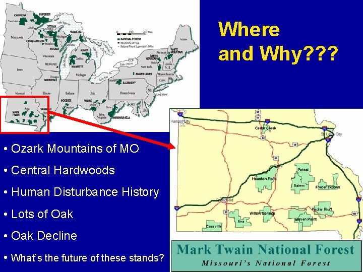
Where and Why? ? ? • Ozark Mountains of MO • Central Hardwoods • Human Disturbance History • Lots of Oak • Oak Decline • What’s the future of these stands?

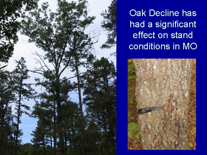
Oak Decline has had a significant effect on stand conditions in MO

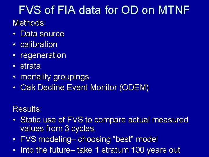
FVS of FIA data for OD on MTNF Methods: • Data source • calibration • regeneration • strata • mortality groupings • Oak Decline Event Monitor (ODEM) Results: • Static use of FVS to compare actual measured values from 3 cycles. • FVS modeling– choosing “best” model • Into the future– take 1 stratum 100 years out

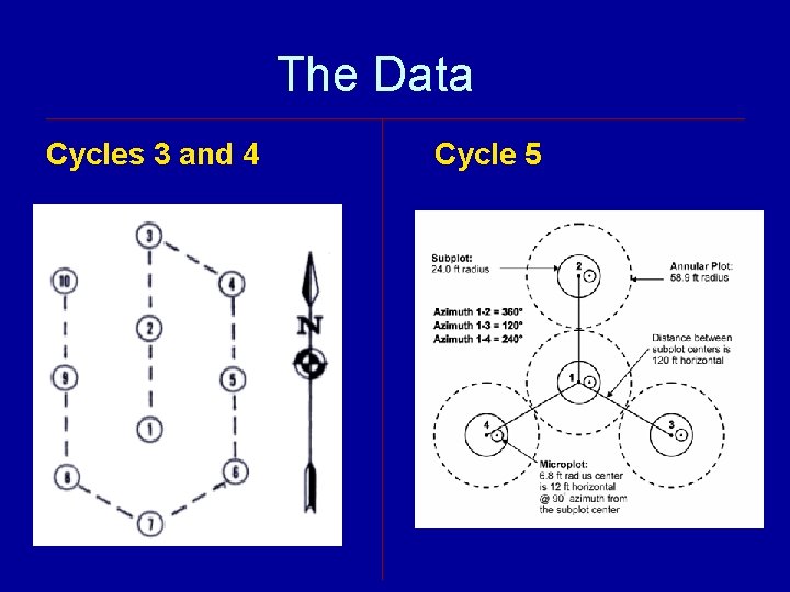
THE DATA • 157 Common stands on the MTNF re-measured in FIA cycles 3 (1976 -1977), 4 (1986 -1987), and 5 (1999 -2003), with the identical center pin. After filtering to exclude disturbed plots, nonoak types, small diameter and other anomalous plots, there were about 100 stands available for analysis. • Data from 911 FIA plots (all oak type) from cycles 3, 4, and 5 on the MTNF were pooled for adjusting max tree and stand growth in FVS.

The Data Cycles 3 and 4 Cycle 5

Calibration of FVS • 557 plots from cycles 3 and 4 used for FVS self-calibration of growth model (Read. Cor. D). ” d re i u q • Defect values to apply in calculation of merchantable volume were based on values which the MTNF used in 2005 Forest Plan Revision. Cycle 4 FIA data was used to determine the allocation of this defect across size classes. • : e M R A y l y b a d m s e Species and size distribution from 911 FIA plots from cycles 3, e s s n 4, and 5 were used to indicate the max size that different tree d A e eto grow, and mortality related to stand species were allowed W basal density index/ area maximums and species distribution. m ointo addfiles (Cap. Size and Adj_OD). These were built S “ • 911 plots used for regeneration imputation… see following slide.

Imputation of Regeneration • Potential tree species for regeneration were divided into 9 possible shade tolerance and max height attainment groups. (for instance: high shade tolerance, mid height attainment group; low shade tolerance, high height attainment group; etc. ) • 911 FIA plots from cycles 3, 4, and 5 were used to determine the typical distribution of advance regeneration (of each of the 9 potential shade tolerance/height attainment groups) under different canopy density and ecological strata. • An “addfile” was created to determine ecological strata and size/density class of each plot and impute the appropriate amount of advance regeneration as saplings from the appropriate shade tolerance/height attainment groups.

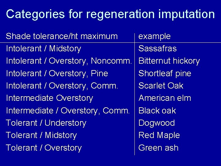
Categories for regeneration imputation Shade tolerance/ht maximum Intolerant / Midstory Intolerant / Overstory, Noncomm. Intolerant / Overstory, Pine Intolerant / Overstory, Comm. Intermediate Overstory Intermediate / Overstory, Comm. Tolerant / Understory Tolerant / Midstory Tolerant / Overstory example Sassafras Bitternut hickory Shortleaf pine Scarlet Oak American elm Black oak Dogwood Red Maple Green ash

Imputation of Regeneration • Potential tree species for regeneration were divided into 9 possible shade tolerance and max height attainment groups. : n o o n n o r i t e t a f 3, 4, and t 911 FIA plots from a cycles 5 were used to u p y distribution a determine thedtypical of advance m I s n r regeneration (of each of the 9 potential shade o u i t h tolerance/height attainment groups) under different a T r e canopy density and ecological strata. n e g e R An “addfile” was created to determine ecological (for instance: high shade tolerance, mid height attainment group; low shade tolerance, high height attainment group; etc. ) • • strata and size/density class of each plot and impute the appropriate amount of advance regeneration as saplings from the appropriate shade tolerance/height attainment groups.

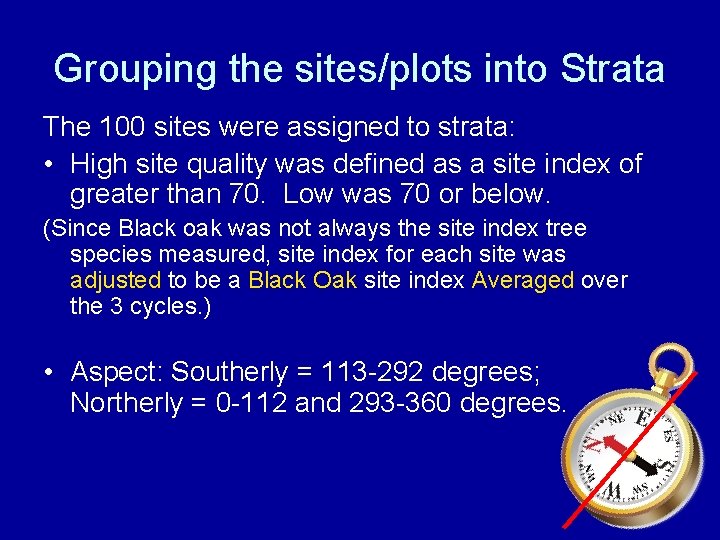
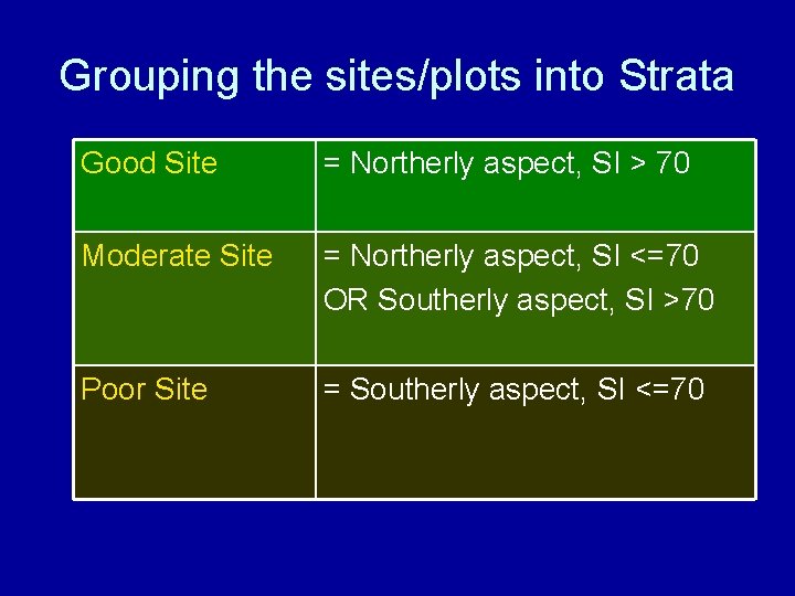
Grouping the sites/plots into Strata The 100 sites were assigned to strata: • High site quality was defined as a site index of greater than 70. Low was 70 or below. (Since Black oak was not always the site index tree species measured, site index for each site was adjusted to be a Black Oak site index Averaged over the 3 cycles. ) • Aspect: Southerly = 113 -292 degrees; Northerly = 0 -112 and 293 -360 degrees.

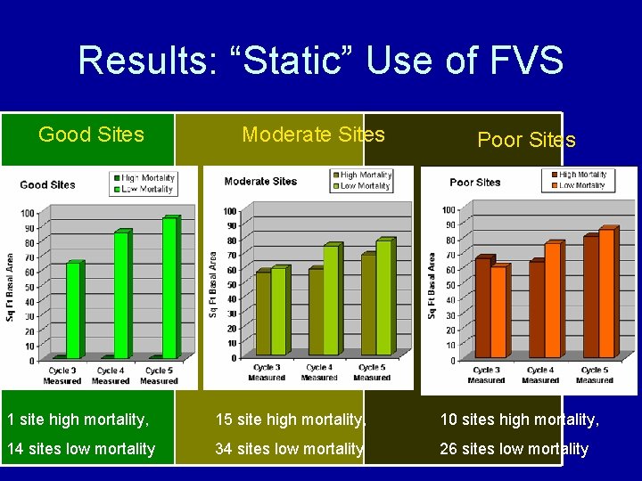
Grouping the sites/plots into Strata Good Site = Northerly aspect, SI > 70 Moderate Site = Northerly aspect, SI <=70 OR Southerly aspect, SI >70 Poor Site = Southerly aspect, SI <=70

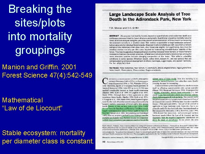
Breaking the sites/plots into mortality groupings Manion and Griffin. 2001 Forest Science 47(4): 542 -549 Mathematical “Law of de Liocourt” Stable ecosystem: mortality per diameter class is constant.

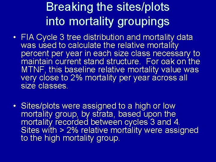
Breaking the sites/plots into mortality groupings • FIA Cycle 3 tree distribution and mortality data was used to calculate the relative mortality percent per year in each size class necessary to maintain current stand structure. For oak on the MTNF, this baseline relative mortality value was very close to 2% mortality per year across all size classes. • Sites/plots were assigned to a high or low mortality group, by strata, based upon the mortality recorded between cycles 3 and 4. Sites with > 2% relative mortality were assigned to the high mortality group.

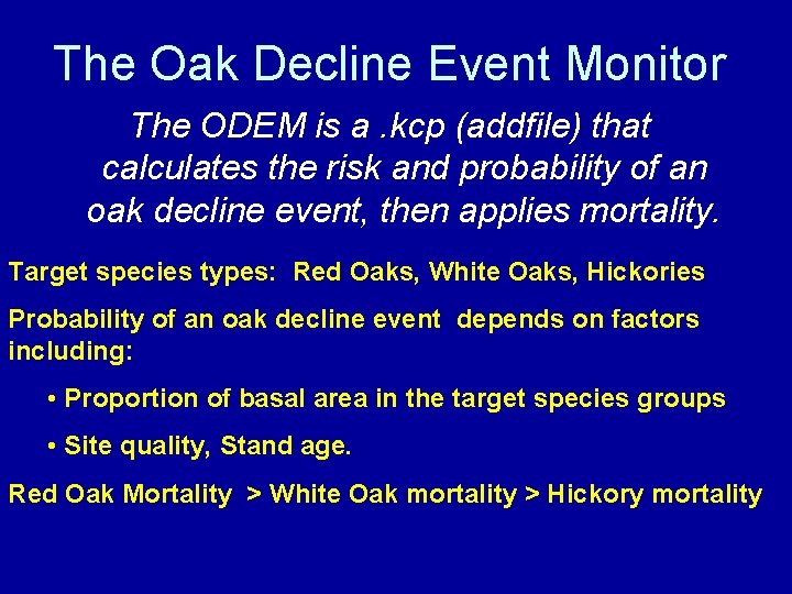
The Oak Decline Event Monitor The ODEM is a. kcp (addfile) that calculates the risk and probability of an oak decline event, then applies mortality. Target species types: Red Oaks, White Oaks, Hickories Probability of an oak decline event depends on factors including: • Proportion of basal area in the target species groups • Site quality, Stand age. Red Oak Mortality > White Oak mortality > Hickory mortality

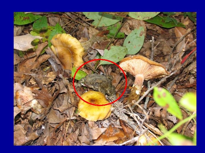
It’s enough to make you want to crawl into your shell and hide.

Results: “Static” Use of FVS Good Sites Moderate Sites Poor Sites 1 site high mortality, 15 site high mortality, 10 sites high mortality, 14 sites low mortality 34 sites low mortality 26 sites low mortality

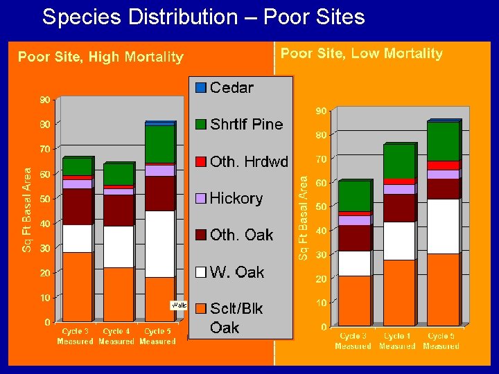
Species Distribution – Poor Sites

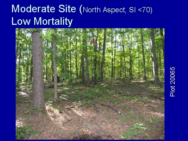
Plot 20065 Moderate Site (North Aspect, SI <70) Low Mortality

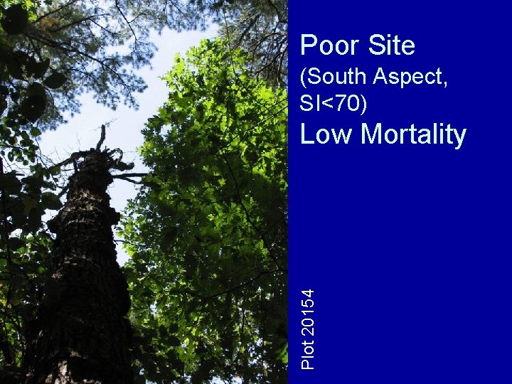
Poor Site (South Aspect, SI<70) Plot 20154 Low Mortality

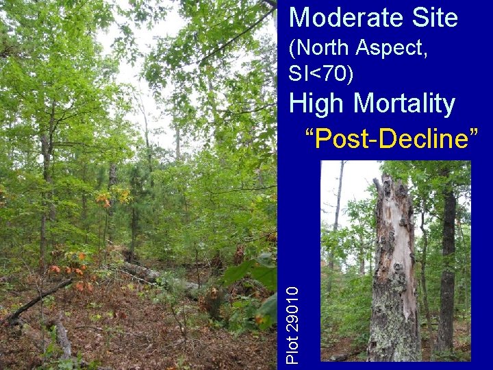
Moderate Site (North Aspect, SI<70) Plot 29010 High Mortality “Post-Decline”

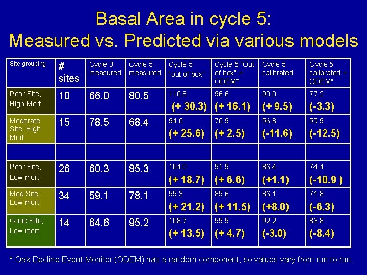
Basal Area in cycle 5: Measured vs. Predicted via various models Site grouping # sites Cycle 3 measured Cycle 5 “out of box” Cycle 5 “Out of box” + ODEM* Cycle 5 calibrated + ODEM* Poor Site, High Mort 10 66. 0 80. 5 110. 8 96. 6 90. 0 77. 2 (+ 9. 5) (-3. 3) Moderate Site, High Mort 15 78. 5 68. 4 94. 0 70. 9 56. 8 55. 9 (+ 25. 6) (+ 2. 5) (-11. 6) (-12. 5) Poor Site, Low mort 26 60. 3 85. 3 104. 0 91. 9 86. 4 74. 4 (+ 18. 7) (+ 6. 6) (+1. 1) (-10. 9 ) Mod Site, Low mort 34 59. 1 78. 1 99. 3 89. 6 86. 1 71. 8 (+ 21. 2) (+ 11. 5) (+8. 0) (-6. 3) Good Site, Low mort 14 64. 6 95. 2 108. 7 99. 9 92. 2 86. 8 (+ 13. 5) (+ 4. 7) (-3. 0) (-8. 4) (+ 30. 3) (+ 16. 1) * Oak Decline Event Monitor (ODEM) has a random component, so values vary from run to run.

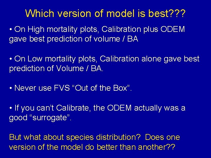
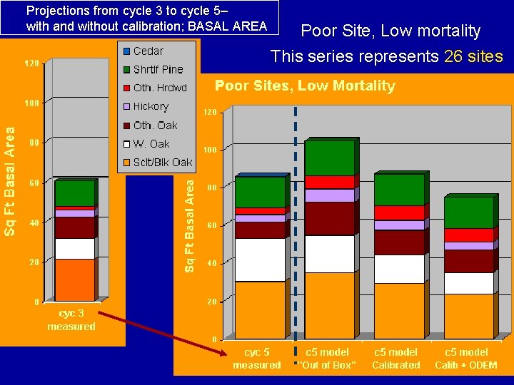
Which version of model is best? ? ? • On High mortality plots, Calibration plus ODEM gave best prediction of volume / BA • On Low mortality plots, Calibration alone gave best prediction of Volume / BA. • Never use FVS “Out of the Box”. • If you can’t Calibrate, the ODEM actually was a good “surrogate”. But what about species distribution? Does one version of the model do better than another? ?

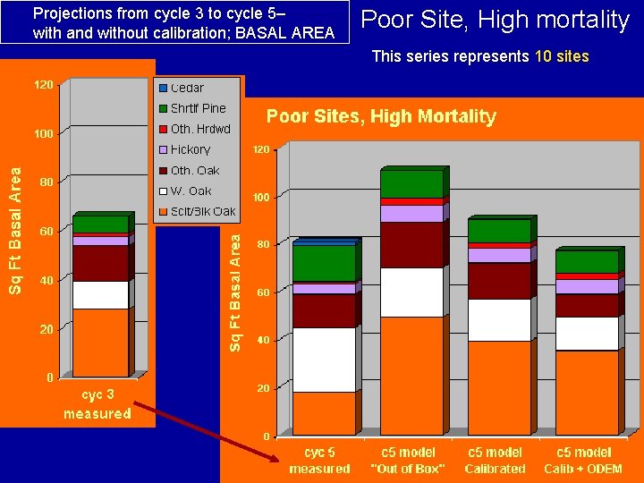
Projections from cycle 3 to cycle 5– with and without calibration; BASAL AREA Poor Site, High mortality This series represents 10 sites

Projections from cycle 3 to cycle 5– with and without calibration; BASAL AREA Poor Site, Low mortality This series represents 26 sites

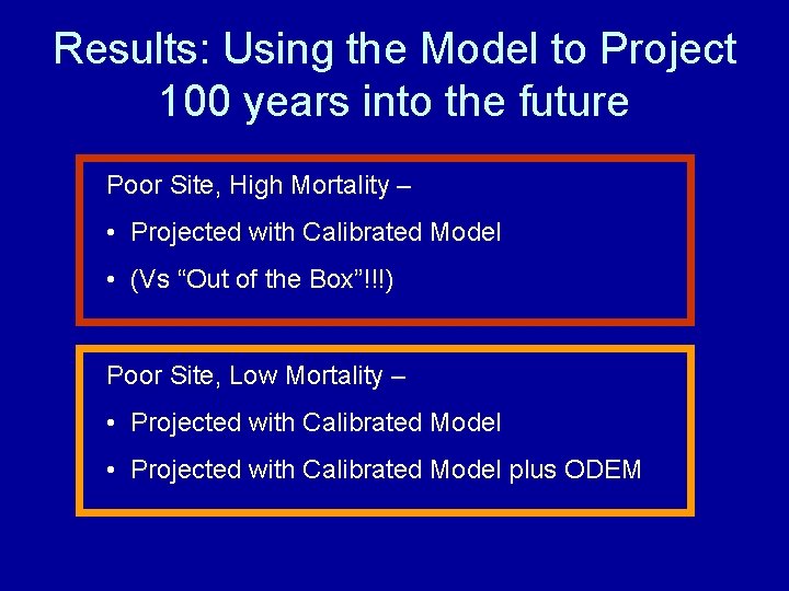
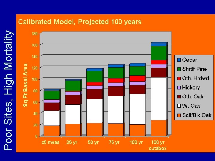
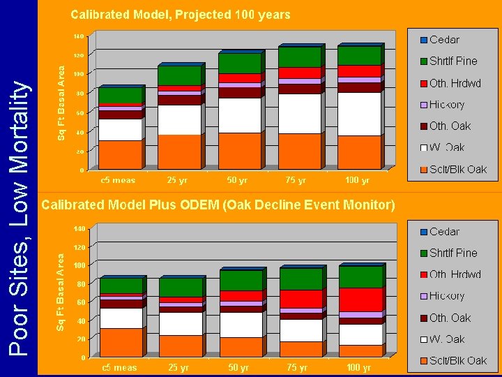
Results: Using the Model to Project 100 years into the future Poor Site, High Mortality – • Projected with Calibrated Model • (Vs “Out of the Box”!!!) Poor Site, Low Mortality – • Projected with Calibrated Model plus ODEM

Poor Sites, High Mortality

Poor Sites, Low Mortality