CMSC 471 Spring 2014 Class 5 Tue 21114

CMSC 471 Spring 2014 Class #5 Tue 2/11/14 Informed Search Professor Marie des. Jardins, mariedj@cs. umbc. edu

HW 2

Outline • Heuristic search • Best-first search – Greedy search – Beam search – A, A* – Examples • Memory-conserving variations of A* • Heuristic functions

Informed Search Chapter 3. 5 -3. 7

Informed Methods Add Domain-Specific Information • Add domain-specific information to select the best path along which to continue searching • Define a heuristic function h(n) that estimates the “goodness” of a node n. – Specifically, h(n) = estimated cost (or distance) of minimal cost path from n to a goal state. • The heuristic function is an estimate of how close we are to a goal, based on domain-specific information that is computable from the current state description.

Heuristics • All domain knowledge used in the search is encoded in the heuristic function h(). • Heuristic search is an example of a “weak method” because of the limited way that domain-specific information is used to solve the problem. • Examples: – Missionaries and Cannibals: Number of people on starting river bank – 8 -puzzle: Number of tiles out of place – 8 -puzzle: Sum of distances each tile is from its goal position • In general: – h(n) ≥ 0 for all nodes n – h(n) = 0 implies that n is a goal node – h(n) = ∞ implies that n is a dead-end that can never lead to a goal

Weak vs. Strong Methods • We use the term weak methods to refer to methods that are extremely general and not tailored to a specific situation. • Examples of weak methods include – Means-ends analysis is a strategy in which we try to represent the current situation and where we want to end up and then look for ways to shrink the differences between the two. – Space splitting is a strategy in which we try to list the possible solutions to a problem and then try to rule out classes of these possibilities. – Subgoaling means to split a large problem into several smaller ones that can be solved one at a time. • Called “weak” methods because they do not take advantage of more powerful domain-specific heuristics

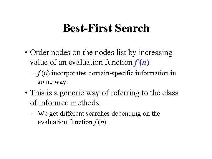
Best-First Search • Order nodes on the nodes list by increasing value of an evaluation function f (n) – f (n) incorporates domain-specific information in some way. • This is a generic way of referring to the class of informed methods. – We get different searches depending on the evaluation function f (n)

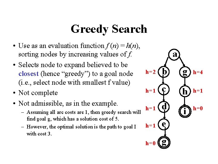
Greedy Search • Use as an evaluation function f (n) = h(n), sorting nodes by increasing values of f. • Selects node to expand believed to be h=2 closest (hence “greedy”) to a goal node (i. e. , select node with smallest f value) h=1 • Not complete • Not admissible, as in the example. h=1 – Assuming all arc costs are 1, then greedy search will find goal g, which has a solution cost of 5. h=1 – However, the optimal solution is the path to goal I with cost 3. h=0 a b g h=4 c h h=1 i h=0 d e g

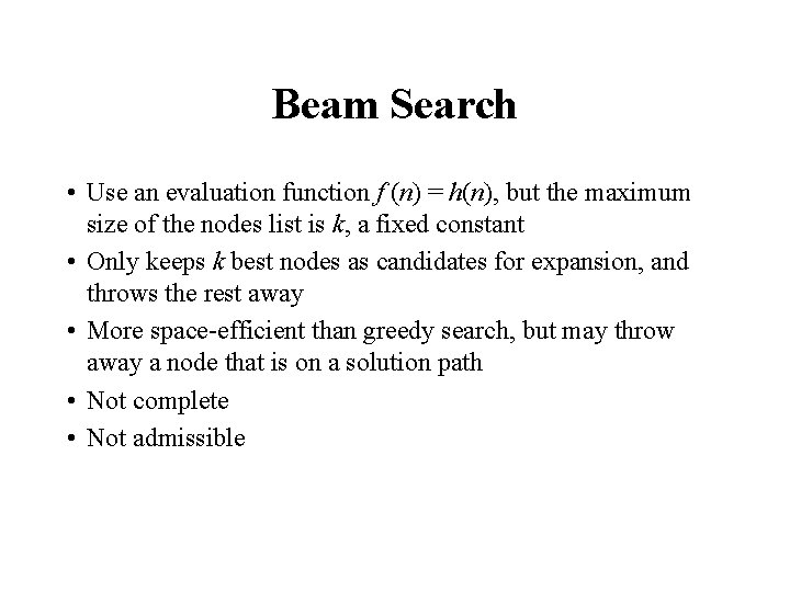
Beam Search • Use an evaluation function f (n) = h(n), but the maximum size of the nodes list is k, a fixed constant • Only keeps k best nodes as candidates for expansion, and throws the rest away • More space-efficient than greedy search, but may throw away a node that is on a solution path • Not complete • Not admissible

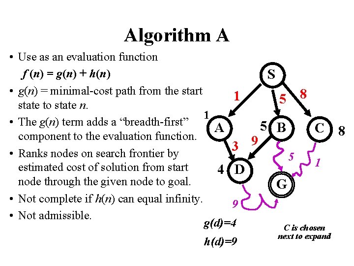
Algorithm A • Use as an evaluation function f (n) = g(n) + h(n) S • g(n) = minimal-cost path from the start 8 1 5 state to state n. 1 • The g(n) term adds a “breadth-first” 5 B A C component to the evaluation function. 9 3 • Ranks nodes on search frontier by 5 1 estimated cost of solution from start 4 D node through the given node to goal. G • Not complete if h(n) can equal infinity. 9 • Not admissible. g(d)=4 C is chosen h(d)=9 next to expand 8

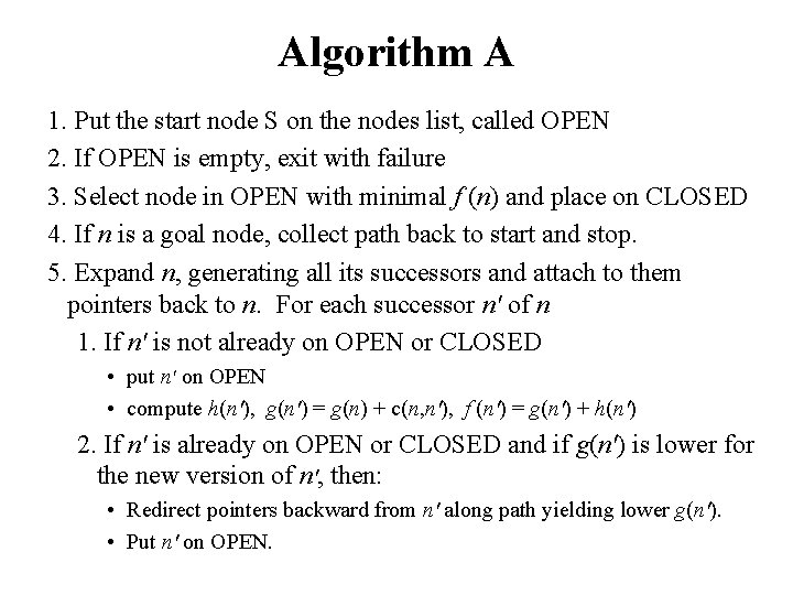
Algorithm A 1. Put the start node S on the nodes list, called OPEN 2. If OPEN is empty, exit with failure 3. Select node in OPEN with minimal f (n) and place on CLOSED 4. If n is a goal node, collect path back to start and stop. 5. Expand n, generating all its successors and attach to them pointers back to n. For each successor n' of n 1. If n' is not already on OPEN or CLOSED • put n' on OPEN • compute h(n'), g(n') = g(n) + c(n, n'), f (n') = g(n') + h(n') 2. If n' is already on OPEN or CLOSED and if g(n') is lower for the new version of n', then: • Redirect pointers backward from n' along path yielding lower g(n'). • Put n' on OPEN.

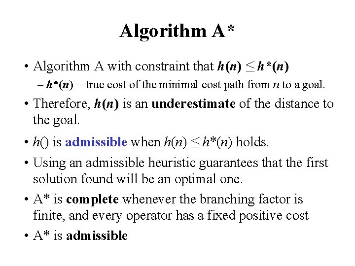
Algorithm A* • Algorithm A with constraint that h(n) ≤ h*(n) – h*(n) = true cost of the minimal cost path from n to a goal. • Therefore, h(n) is an underestimate of the distance to the goal. • h() is admissible when h(n) ≤ h*(n) holds. • Using an admissible heuristic guarantees that the first solution found will be an optimal one. • A* is complete whenever the branching factor is finite, and every operator has a fixed positive cost • A* is admissible

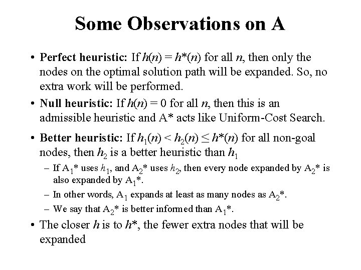
Some Observations on A • Perfect heuristic: If h(n) = h*(n) for all n, then only the nodes on the optimal solution path will be expanded. So, no extra work will be performed. • Null heuristic: If h(n) = 0 for all n, then this is an admissible heuristic and A* acts like Uniform-Cost Search. • Better heuristic: If h 1(n) < h 2(n) ≤ h*(n) for all non-goal nodes, then h 2 is a better heuristic than h 1 – If A 1* uses h 1, and A 2* uses h 2, then every node expanded by A 2* is also expanded by A 1*. – In other words, A 1 expands at least as many nodes as A 2*. – We say that A 2* is better informed than A 1*. • The closer h is to h*, the fewer extra nodes that will be expanded

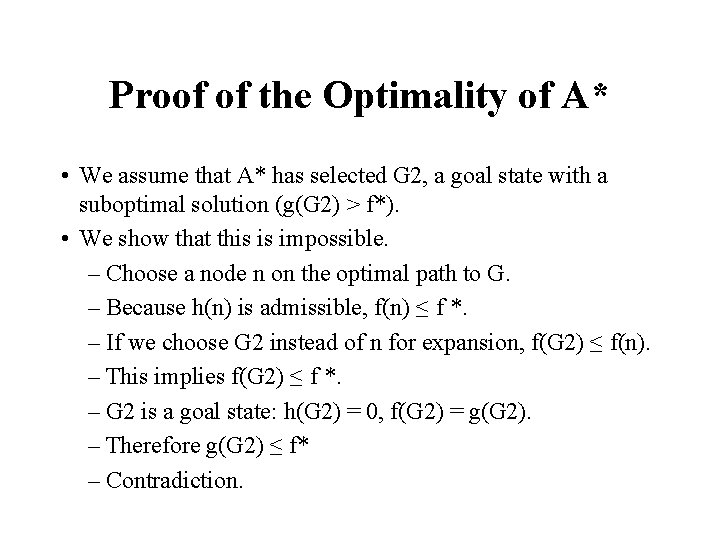
Proof of the Optimality of A* • We assume that A* has selected G 2, a goal state with a suboptimal solution (g(G 2) > f*). • We show that this is impossible. – Choose a node n on the optimal path to G. – Because h(n) is admissible, f(n) ≤ f *. – If we choose G 2 instead of n for expansion, f(G 2) ≤ f(n). – This implies f(G 2) ≤ f *. – G 2 is a goal state: h(G 2) = 0, f(G 2) = g(G 2). – Therefore g(G 2) ≤ f* – Contradiction.

Dealing with Hard Problems • For large problems, A* often requires too much space. • Two variations conserve memory: IDA* and SMA* • IDA* -- iterative deepening A* – uses successive iteration with growing limits on f. For example, • A* but don’t consider any node n where f (n) > 10 • A* but don’t consider any node n where f (n) > 20 • A* but don’t consider any node n where f (n) > 30, . . . • SMA* -- Simplified Memory-Bounded A* – uses a queue of restricted size to limit memory use. – throws away the “oldest” worst solution.

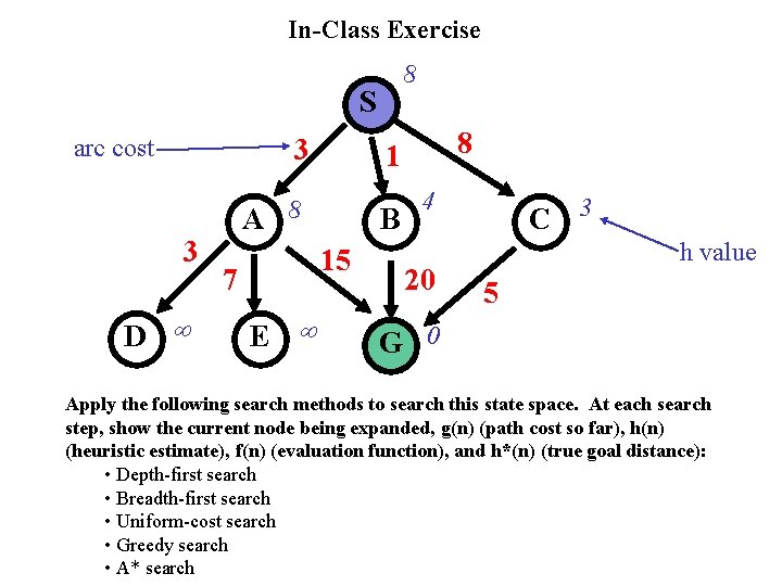
In-Class Exercise 8 S 3 arc cost 3 D A 8 B 15 7 E 8 1 4 20 C 3 h value 5 G 0 Apply the following search methods to search this state space. At each search step, show the current node being expanded, g(n) (path cost so far), h(n) (heuristic estimate), f(n) (evaluation function), and h*(n) (true goal distance): • Depth-first search • Breadth-first search • Uniform-cost search • Greedy search • A* search

What’s a Good Heuristic? • If h 1(n) < h 2(n) ≤ h*(n) for all n, h 2 is better than (dominates) h 1. • Relaxing the problem: remove constraints to create a (much) easier problem; use the solution cost for this problem as the heuristic function • Combining heuristics: take the max of several admissible heuristics: still have an admissible heuristic, and it’s better! • Use statistical estimates to compute h: may lose admissibility • Identify good features, then use a learning algorithm to find a heuristic function: also may lose admissibility

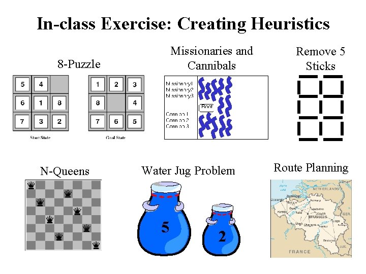
In-class Exercise: Creating Heuristics Missionaries and Cannibals 8 -Puzzle N-Queens Water Jug Problem 5 2 Remove 5 Sticks Route Planning

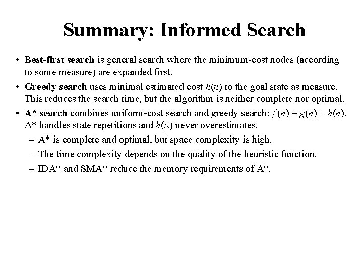
Summary: Informed Search • Best-first search is general search where the minimum-cost nodes (according to some measure) are expanded first. • Greedy search uses minimal estimated cost h(n) to the goal state as measure. This reduces the search time, but the algorithm is neither complete nor optimal. • A* search combines uniform-cost search and greedy search: f (n) = g(n) + h(n). A* handles state repetitions and h(n) never overestimates. – A* is complete and optimal, but space complexity is high. – The time complexity depends on the quality of the heuristic function. – IDA* and SMA* reduce the memory requirements of A*.