CHAPTER 4 Parametric Methods Parametric Estimation n n

CHAPTER 4: Parametric Methods

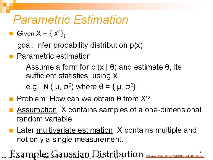
Parametric Estimation n n Given X = { xt }t goal: infer probability distribution p(x) Parametric estimation: Assume a form for p (x | θ) and estimate θ, its sufficient statistics, using X e. g. , N ( μ, σ2) where θ = { μ, σ2} Problem: How can we obtain θ from X? Assumption: X contains samples of a one-dimensional random variable Later multivariate estimation: X contains multiple and not only a single measurement. Example; Gaussian Distribution Lecture Notes for E Alpaydın 2004 Introduction to Machine Learning © The MIT Press (V 1. 1) 2 http: //en. wikipedia. org/wiki/Normal_distribution

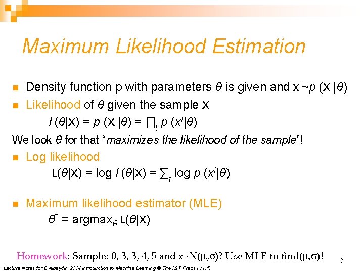
Maximum Likelihood Estimation n n Density function p with parameters θ is given and xt~p (X |θ) Likelihood of θ given the sample X l (θ|X) = p (X |θ) = ∏t p (xt|θ) We look θ for that “maximizes the likelihood of the sample”! n Log likelihood L(θ|X) = log l (θ|X) = ∑t log p (xt|θ) n Maximum likelihood estimator (MLE) θ* = argmaxθ L(θ|X) Homework: Sample: 0, 3, 3, 4, 5 and x~N( , )? Use MLE to find( , )! Lecture Notes for E Alpaydın 2004 Introduction to Machine Learning © The MIT Press (V 1. 1) 3

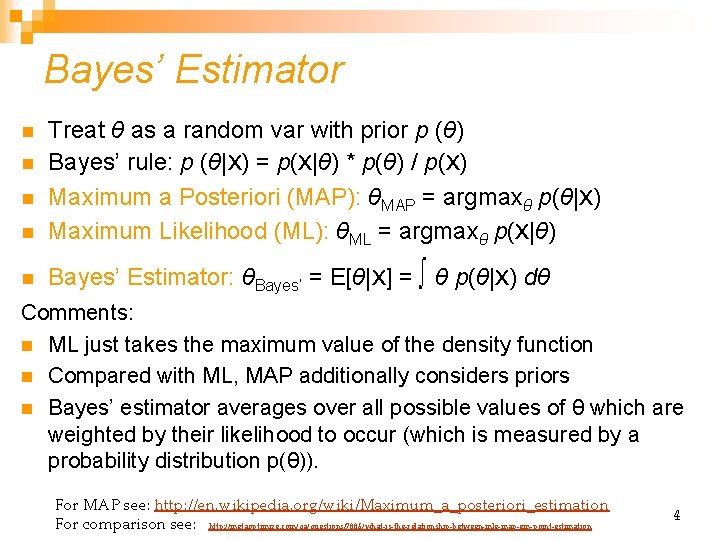
Bayes’ Estimator n Treat θ as a random var with prior p (θ) Bayes’ rule: p (θ|X) = p(X|θ) * p(θ) / p(X) Maximum a Posteriori (MAP): θMAP = argmaxθ p(θ|X) Maximum Likelihood (ML): θML = argmaxθ p(X|θ) n Bayes’ Estimator: θBayes’ = E[θ|X] = ∫ θ p(θ|X) dθ n n n Comments: n ML just takes the maximum value of the density function n Compared with ML, MAP additionally considers priors n Bayes’ estimator averages over all possible values of θ which are weighted by their likelihood to occur (which is measured by a probability distribution p(θ)). For MAP see: http: //en. wikipedia. org/wiki/Maximum_a_posteriori_estimation For comparison see: http: //metaoptimize. com/qa/questions/7885/what-is-the-relationship-between-mle-map-em-point-estimation 4

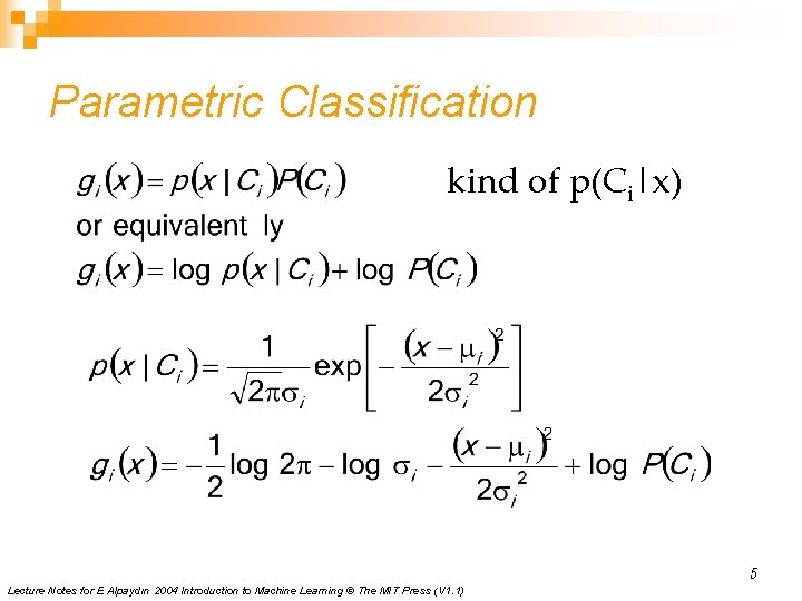
Parametric Classification kind of p(Ci|x) 5 Lecture Notes for E Alpaydın 2004 Introduction to Machine Learning © The MIT Press (V 1. 1)

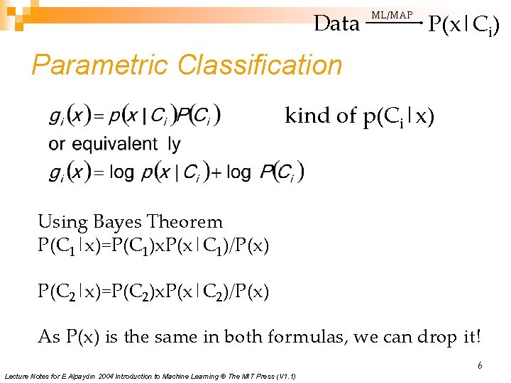
Data ML/MAP P(x|Ci) Parametric Classification kind of p(Ci|x) Using Bayes Theorem P(C 1|x)=P(C 1)x. P(x|C 1)/P(x) P(C 2|x)=P(C 2)x. P(x|C 2)/P(x) As P(x) is the same in both formulas, we can drop it! 6 Lecture Notes for E Alpaydın 2004 Introduction to Machine Learning © The MIT Press (V 1. 1)

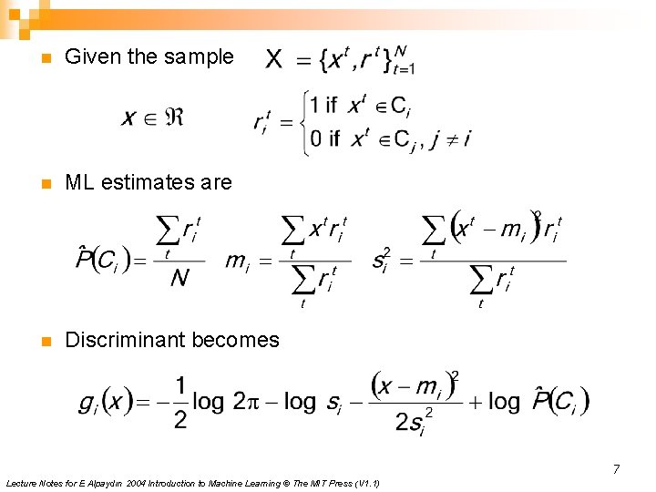
n Given the sample n ML estimates are n Discriminant becomes 7 Lecture Notes for E Alpaydın 2004 Introduction to Machine Learning © The MIT Press (V 1. 1)

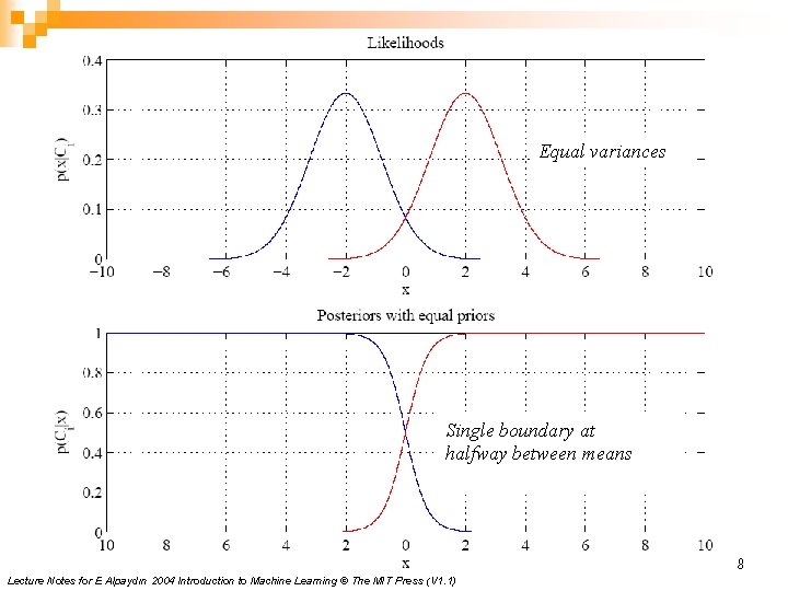
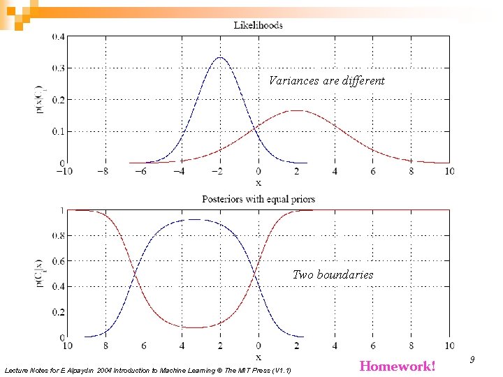
Equal variances Single boundary at halfway between means 8 Lecture Notes for E Alpaydın 2004 Introduction to Machine Learning © The MIT Press (V 1. 1)

Variances are different Two boundaries Lecture Notes for E Alpaydın 2004 Introduction to Machine Learning © The MIT Press (V 1. 1) Homework! 9

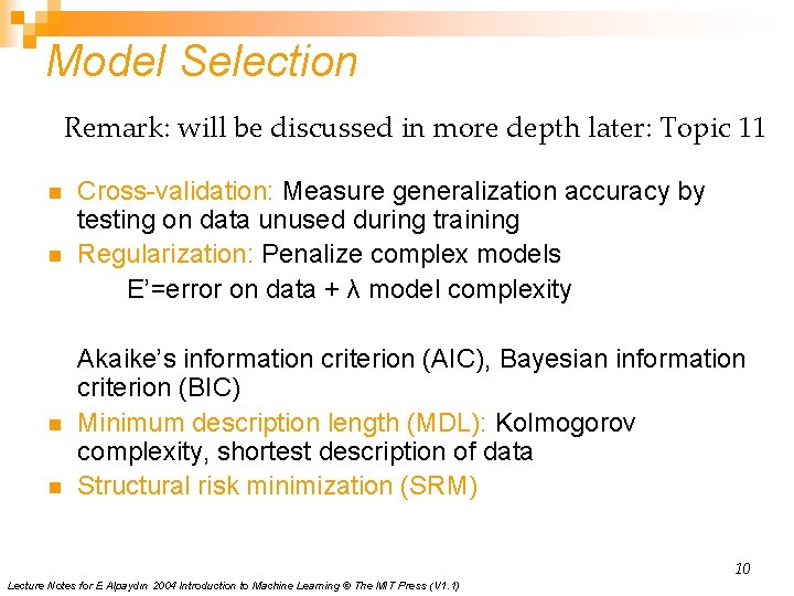
Model Selection Remark: will be discussed in more depth later: Topic 11 n n Cross-validation: Measure generalization accuracy by testing on data unused during training Regularization: Penalize complex models E’=error on data + λ model complexity Akaike’s information criterion (AIC), Bayesian information criterion (BIC) Minimum description length (MDL): Kolmogorov complexity, shortest description of data Structural risk minimization (SRM) 10 Lecture Notes for E Alpaydın 2004 Introduction to Machine Learning © The MIT Press (V 1. 1)

CHAPTER 5: Multivariate Methods Normal Distribution: http: //en. wikipedia. org/wiki/Normal_distribution Z-score: see http: //en. wikipedia. org/wiki/Standard_score

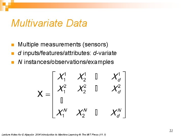
Multivariate Data n n n Multiple measurements (sensors) d inputs/features/attributes: d-variate N instances/observations/examples 12 Lecture Notes for E Alpaydın 2004 Introduction to Machine Learning © The MIT Press (V 1. 1)

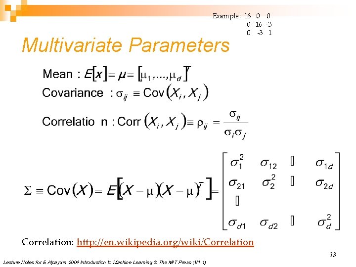
Example: 16 0 0 0 16 -3 0 -3 1 Multivariate Parameters Correlation: http: //en. wikipedia. org/wiki/Correlation 13 Lecture Notes for E Alpaydın 2004 Introduction to Machine Learning © The MIT Press (V 1. 1)

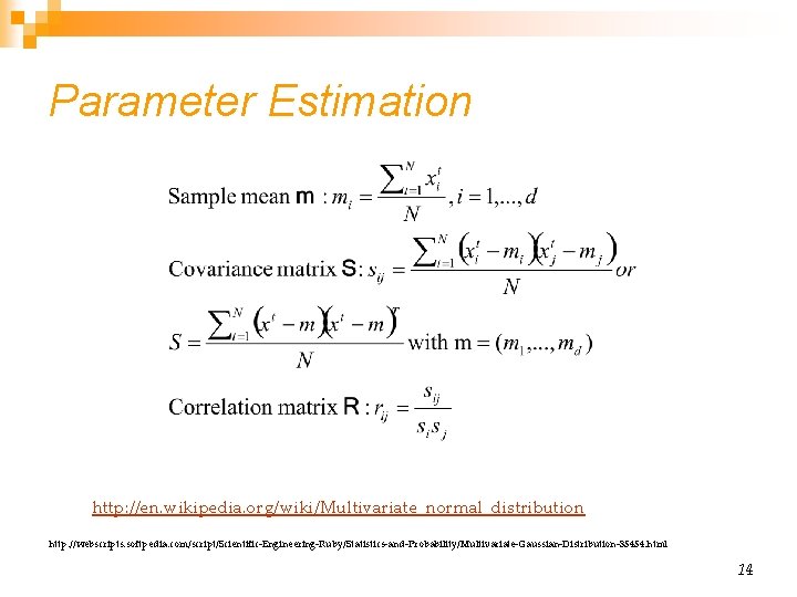
Parameter Estimation http: //en. wikipedia. org/wiki/Multivariate_normal_distribution http: //webscripts. softpedia. com/script/Scientific-Engineering-Ruby/Statistics-and-Probability/Multivariate-Gaussian-Distribution-35454. html 14

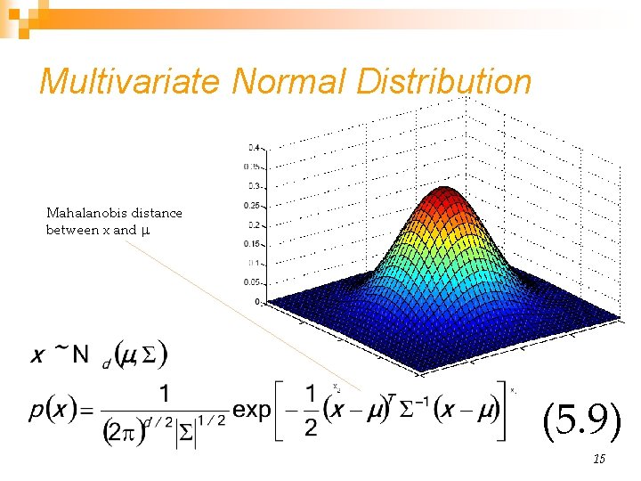
Multivariate Normal Distribution Mahalanobis distance between x and (5. 9) 15

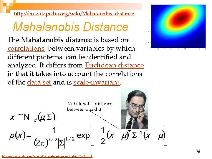
http: //en. wikipedia. org/wiki/Mahalanobis_distance Mahalanobis Distance The Mahalanobis distance is based on correlations between variables by which different patterns can be identified analyzed. It differs from Euclidean distance in that it takes into account the correlations of the data set and is scale-invariant. Mahalanobis distance between x and http: //www. analyzemath. com/Calculators/inverse_matrix_3 by 3. html 16

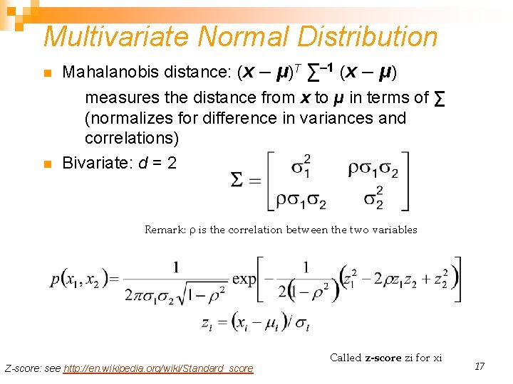
Multivariate Normal Distribution n n Mahalanobis distance: (x – μ)T ∑– 1 (x – μ) measures the distance from x to μ in terms of ∑ (normalizes for difference in variances and correlations) Bivariate: d = 2 Remark: is the correlation between the two variables Z-score: see http: //en. wikipedia. org/wiki/Standard_score Called z-score zi for xi 17

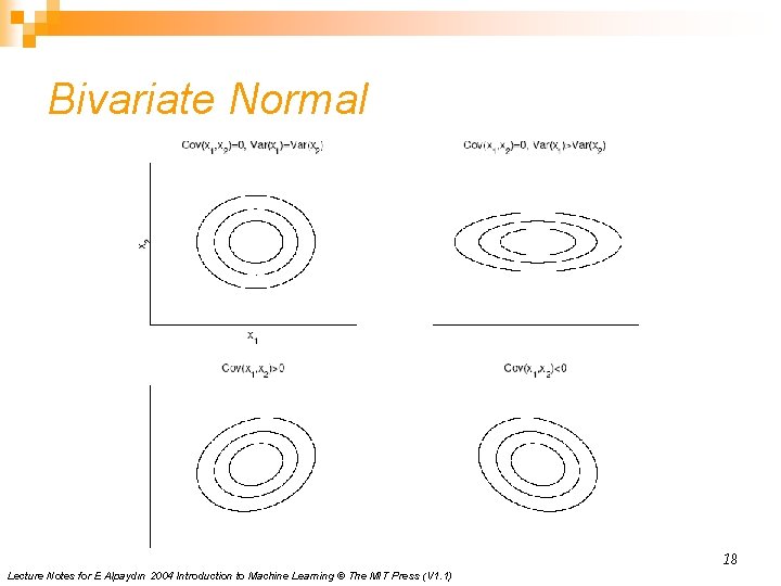
Bivariate Normal 18 Lecture Notes for E Alpaydın 2004 Introduction to Machine Learning © The MIT Press (V 1. 1)

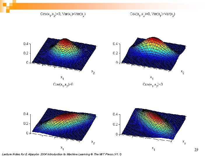
19 Lecture Notes for E Alpaydın 2004 Introduction to Machine Learning © The MIT Press (V 1. 1)

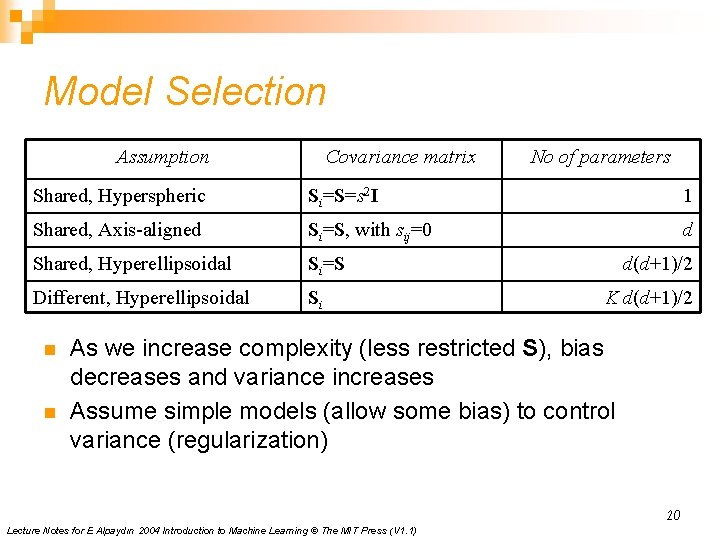
Model Selection Assumption Covariance matrix No of parameters Shared, Hyperspheric Si=S=s 2 I 1 Shared, Axis-aligned Si=S, with sij=0 d Shared, Hyperellipsoidal Si=S Different, Hyperellipsoidal Si n n d(d+1)/2 K d(d+1)/2 As we increase complexity (less restricted S), bias decreases and variance increases Assume simple models (allow some bias) to control variance (regularization) 20 Lecture Notes for E Alpaydın 2004 Introduction to Machine Learning © The MIT Press (V 1. 1)