Chapter 3 pp 101 152 William J Pervin

Chapter 3 pp. 101 -152 William J. Pervin The University of Texas at Dallas Richardson, Texas 75083 The Erik Jonsson School of Engineering and Computer Science

Chapter 3 Continuous Random Variables The Erik Jonsson School of Engineering and Computer Science

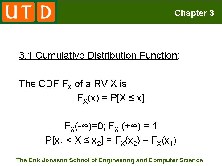
Chapter 3 3. 1 Cumulative Distribution Function: The CDF FX of a RV X is FX(x) = P[X ≤ x] FX(-∞)=0; FX (+∞) = 1 P[x 1 < X ≤ x 2] = FX(x 2) – FX(x 1) The Erik Jonsson School of Engineering and Computer Science

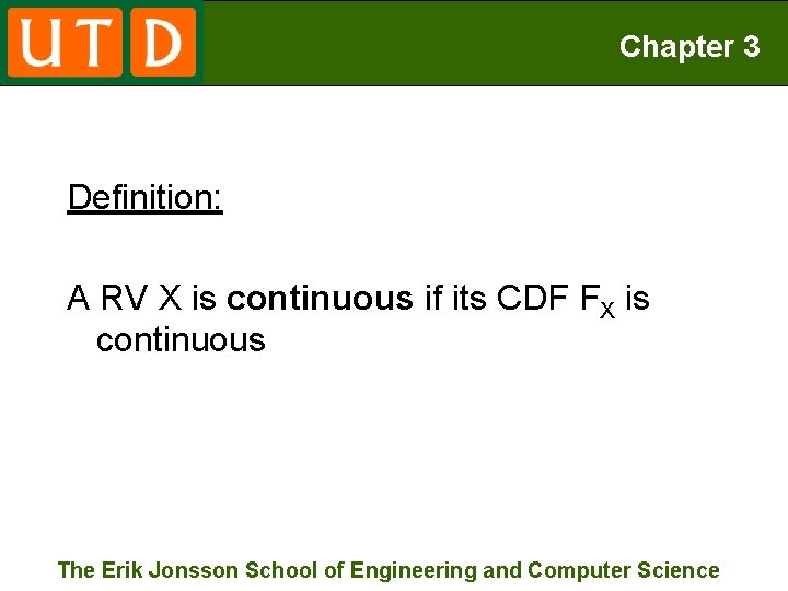
Chapter 3 Definition: A RV X is continuous if its CDF FX is continuous The Erik Jonsson School of Engineering and Computer Science

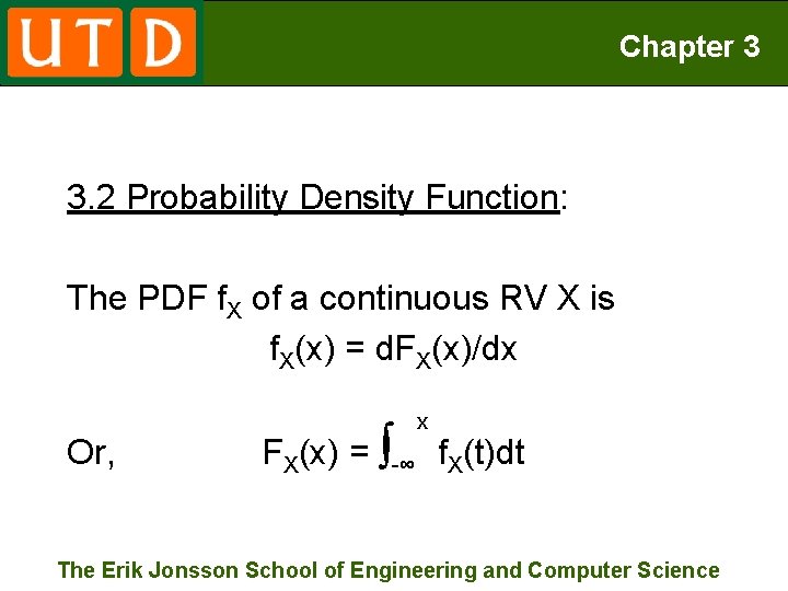
Chapter 3 3. 2 Probability Density Function: The PDF f. X of a continuous RV X is f. X(x) = d. FX(x)/dx Or, x FX(x) = ∫-∞ f. X(t)dt The Erik Jonsson School of Engineering and Computer Science

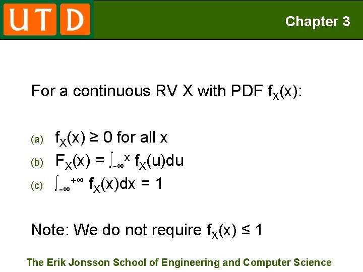
Chapter 3 For a continuous RV X with PDF f. X(x): (a) (b) (c) f. X(x) ≥ 0 for all x FX(x) = ∫-∞x f. X(u)du ∫-∞+∞ f. X(x)dx = 1 Note: We do not require f. X(x) ≤ 1 The Erik Jonsson School of Engineering and Computer Science

Chapter 3 x 2 P[x 1 < X ≤ x 2] = ∫x 1 f. X(x)dx Note that endpoints don’t matter! The Erik Jonsson School of Engineering and Computer Science

Chapter 3 3. 3 Expected Values: E[X] = ∫ xf. X(x)dx = μX E[g(X)] = ∫ g(x)f. X(x)dx Var[X] = ∫ (x - μX)2 f. X(x) dx The Erik Jonsson School of Engineering and Computer Science

Chapter 3 E[X – μX] = 0; that is, μX = E[X] E[a. X + b] = a. E[X] + b Var[X] = E[X 2] – μX 2 Var[a. X + b] = a 2 Var[X] Thus, σa. X+b = aσX The Erik Jonsson School of Engineering and Computer Science

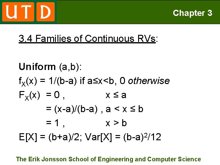
Chapter 3 3. 4 Families of Continuous RVs: Uniform (a, b): f. X(x) = 1/(b-a) if a≤x<b, 0 otherwise FX(x) = 0 , x≤a = (x-a)/(b-a) , a < x ≤ b =1, x>b E[X] = (b+a)/2; Var[X] = (b-a)2/12 The Erik Jonsson School of Engineering and Computer Science

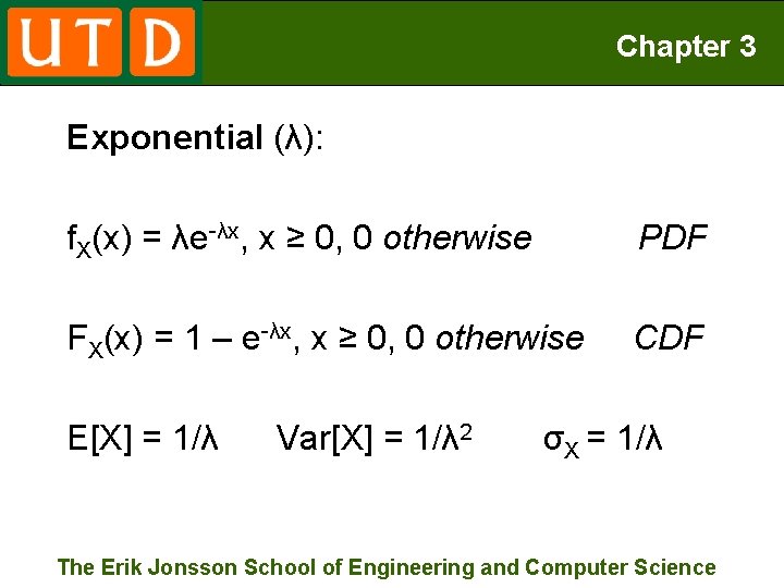
Chapter 3 Exponential (λ): f. X(x) = λe-λx, x ≥ 0, 0 otherwise PDF FX(x) = 1 – e-λx, x ≥ 0, 0 otherwise CDF E[X] = 1/λ Var[X] = 1/λ 2 σX = 1/λ The Erik Jonsson School of Engineering and Computer Science

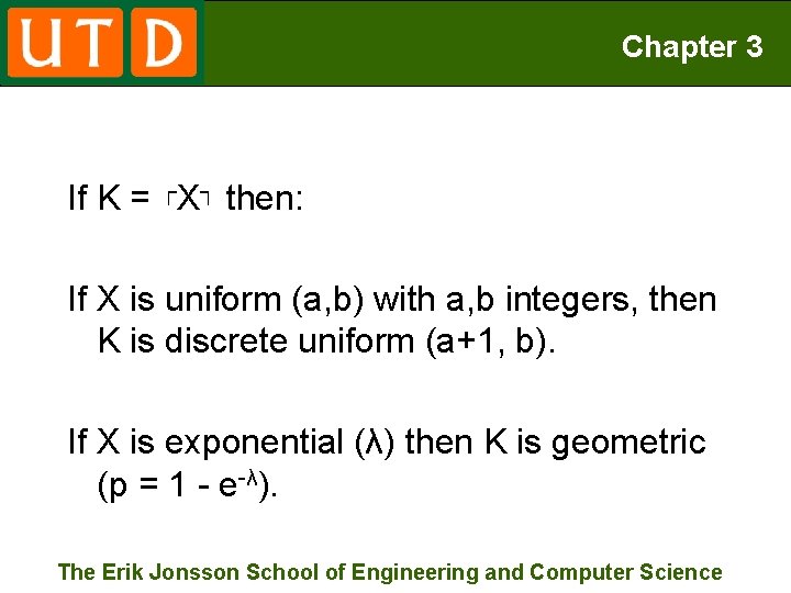
Chapter 3 If K = ┌X┐ then: If X is uniform (a, b) with a, b integers, then K is discrete uniform (a+1, b). If X is exponential (λ) then K is geometric (p = 1 - e-λ). The Erik Jonsson School of Engineering and Computer Science

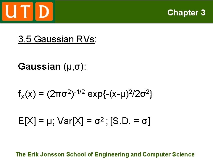
Chapter 3 3. 5 Gaussian RVs: Gaussian (μ, σ): f. X(x) = (2πσ2)-1/2 exp{-(x-μ)2/2σ2} E[X] = μ; Var[X] = σ2 ; [S. D. = σ] The Erik Jonsson School of Engineering and Computer Science

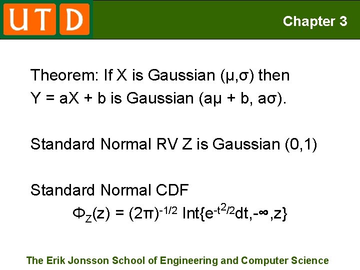
Chapter 3 Theorem: If X is Gaussian (μ, σ) then Y = a. X + b is Gaussian (aμ + b, aσ). Standard Normal RV Z is Gaussian (0, 1) Standard Normal CDF 2/2 -1/2 -t ΦZ(z) = (2π) Int{e dt, -∞, z} The Erik Jonsson School of Engineering and Computer Science

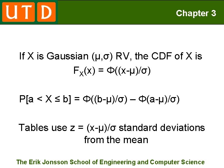
Chapter 3 If X is Gaussian (μ, σ) RV, the CDF of X is FX(x) = Φ((x-μ)/σ) P[a < X ≤ b] = Φ((b-μ)/σ) – Φ(a-μ)/σ) Tables use z = (x-μ)/σ standard deviations from the mean The Erik Jonsson School of Engineering and Computer Science

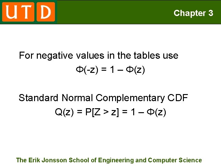
Chapter 3 For negative values in the tables use Φ(-z) = 1 – Φ(z) Standard Normal Complementary CDF Q(z) = P[Z > z] = 1 – Φ(z) The Erik Jonsson School of Engineering and Computer Science

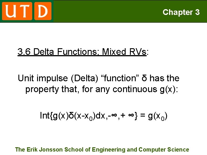
Chapter 3 3. 6 Delta Functions; Mixed RVs: Unit impulse (Delta) “function” δ has the property that, for any continuous g(x): Int{g(x)δ(x-x 0)dx, -∞, + ∞} = g(x 0) The Erik Jonsson School of Engineering and Computer Science

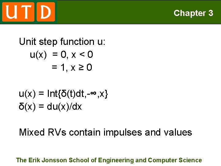
Chapter 3 Unit step function u: u(x) = 0, x < 0 = 1, x ≥ 0 u(x) = Int{δ(t)dt, -∞, x} δ(x) = du(x)/dx Mixed RVs contain impulses and values The Erik Jonsson School of Engineering and Computer Science

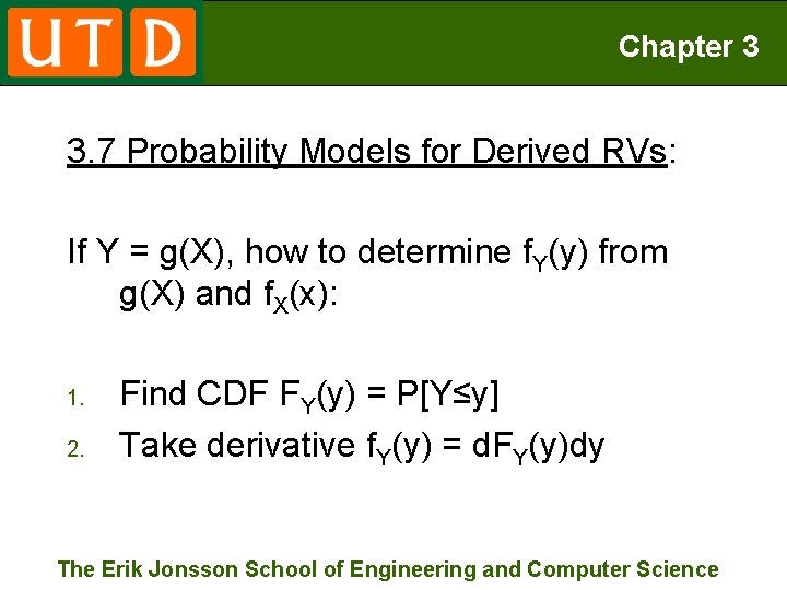
Chapter 3 3. 7 Probability Models for Derived RVs: If Y = g(X), how to determine f. Y(y) from g(X) and f. X(x): 1. 2. Find CDF FY(y) = P[Y≤y] Take derivative f. Y(y) = d. FY(y)dy The Erik Jonsson School of Engineering and Computer Science

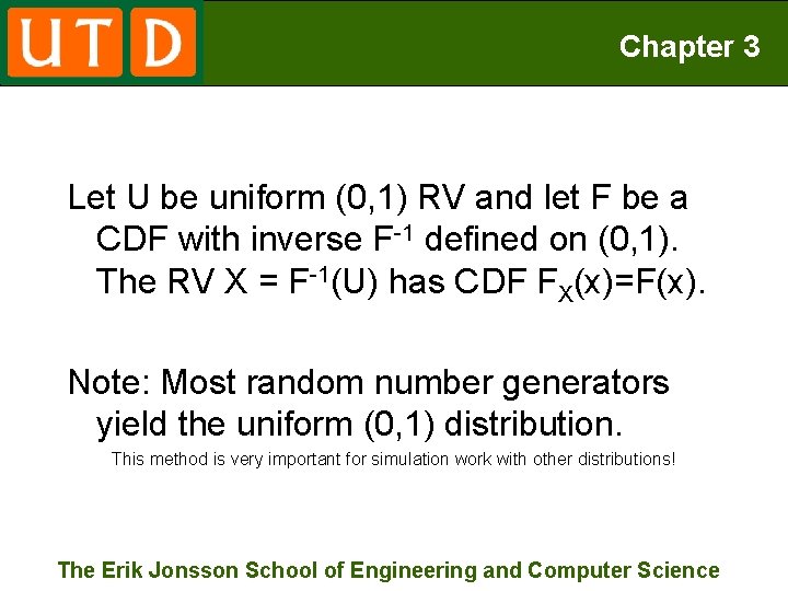
Chapter 3 Let U be uniform (0, 1) RV and let F be a CDF with inverse F-1 defined on (0, 1). The RV X = F-1(U) has CDF FX(x)=F(x). Note: Most random number generators yield the uniform (0, 1) distribution. This method is very important for simulation work with other distributions! The Erik Jonsson School of Engineering and Computer Science

Chapter 3 3. 8 Conditioning a Continuous RV 3. 9 MATLAB The Erik Jonsson School of Engineering and Computer Science