Chapter 16 TimeSeries Forecasting Yandell Econ 216 Chap

Chapter 16 Time-Series Forecasting Yandell – Econ 216 Chap 16 -1

Chapter Goals After completing this chapter, you should be able to: n Develop and implement basic forecasting models n Identify the components present in a time series n n Use smoothing-based forecasting models, including single exponential smoothing Apply trend-based forecasting models, including linear trend, nonlinear trend, and seasonally adjusted trend Yandell – Econ 216 Chap 16 -2

The Importance of Forecasting n n Governments forecast unemployment, interest rates, and expected revenues from income taxes for policy purposes Marketing executives forecast demand, sales, and consumer preferences for strategic planning College administrators forecast enrollments to plan for facilities and for faculty recruitment Retail stores forecast demand to control inventory levels, hire employees and provide training Yandell – Econ 216 Chap 16 -3

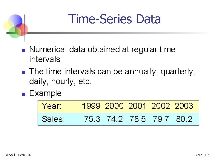
Time-Series Data n n n Numerical data obtained at regular time intervals The time intervals can be annually, quarterly, daily, hourly, etc. Example: Yandell – Econ 216 Year: 1999 2000 2001 2002 2003 Sales: 75. 3 74. 2 78. 5 79. 7 80. 2 Chap 16 -4

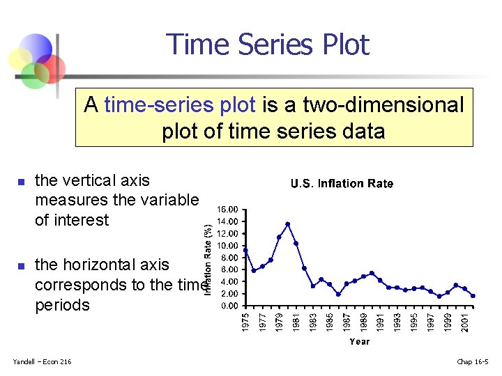
Time Series Plot A time-series plot is a two-dimensional plot of time series data n n the vertical axis measures the variable of interest the horizontal axis corresponds to the time periods Yandell – Econ 216 Chap 16 -5

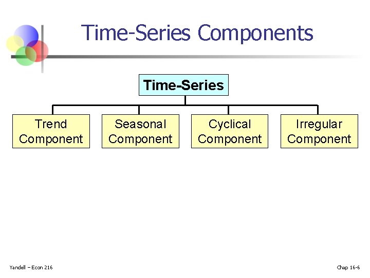
Time-Series Components Time-Series Trend Component Yandell – Econ 216 Seasonal Component Cyclical Component Irregular Component Chap 16 -6

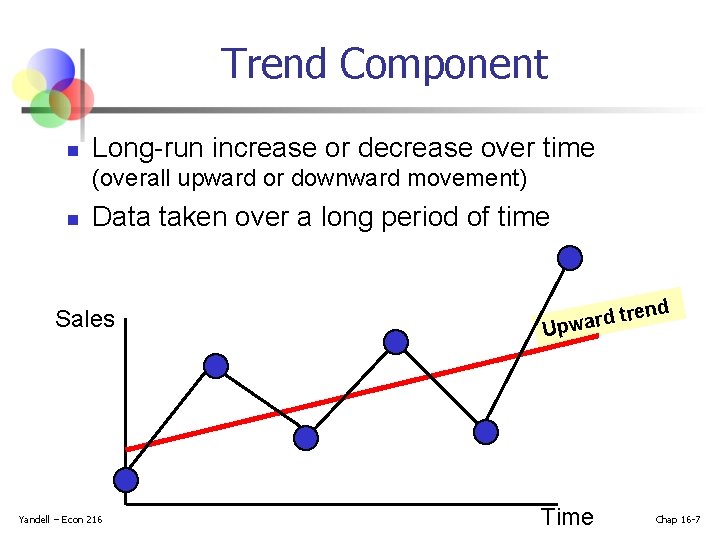
Trend Component n Long-run increase or decrease over time (overall upward or downward movement) n Data taken over a long period of time Sales Yandell – Econ 216 d ren t d r a pw U Time Chap 16 -7

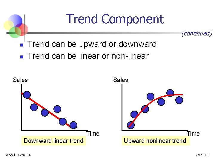
Trend Component (continued) n n Trend can be upward or downward Trend can be linear or non-linear Sales Time Downward linear trend Yandell – Econ 216 Time Upward nonlinear trend Chap 16 -8

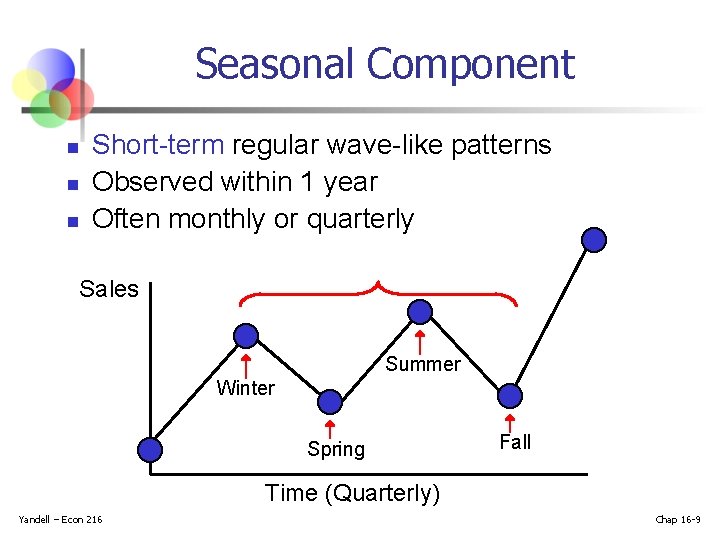
Seasonal Component n n n Short-term regular wave-like patterns Observed within 1 year Often monthly or quarterly Sales Summer Winter Spring Fall Time (Quarterly) Yandell – Econ 216 Chap 16 -9

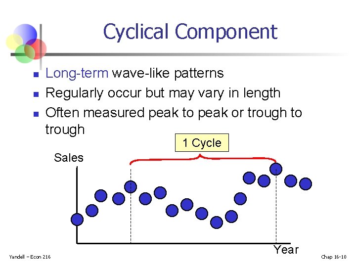
Cyclical Component n n n Long-term wave-like patterns Regularly occur but may vary in length Often measured peak to peak or trough to trough 1 Cycle Sales Yandell – Econ 216 Year Chap 16 -10

Irregular Component n n Unpredictable, random, “residual” fluctuations Due to random variations of n n n Yandell – Econ 216 Nature Accidents or unusual events “Noise” in the time series Chap 16 -11

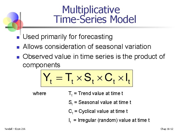
Multiplicative Time-Series Model n n n Used primarily forecasting Allows consideration of seasonal variation Observed value in time series is the product of components where Tt = Trend value at time t St = Seasonal value at time t Ct = Cyclical value at time t It = Irregular (random) value at time t Yandell – Econ 216 Chap 16 -12

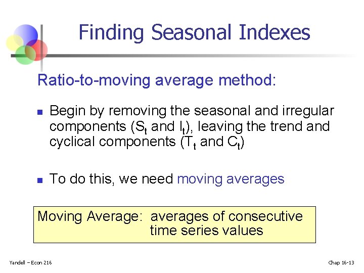
Finding Seasonal Indexes Ratio-to-moving average method: n n Begin by removing the seasonal and irregular components (St and It), leaving the trend and cyclical components (Tt and Ct) To do this, we need moving averages Moving Average: averages of consecutive time series values Yandell – Econ 216 Chap 16 -13

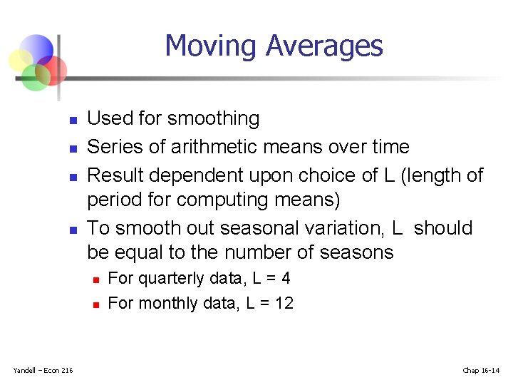
Moving Averages n n Used for smoothing Series of arithmetic means over time Result dependent upon choice of L (length of period for computing means) To smooth out seasonal variation, L should be equal to the number of seasons n n Yandell – Econ 216 For quarterly data, L = 4 For monthly data, L = 12 Chap 16 -14

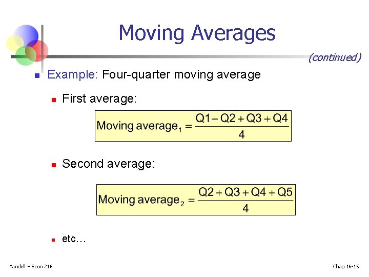
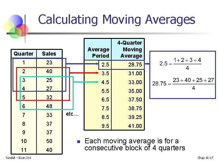
Moving Averages (continued) n Example: Four-quarter moving average n First average: n Second average: n etc… Yandell – Econ 216 Chap 16 -15

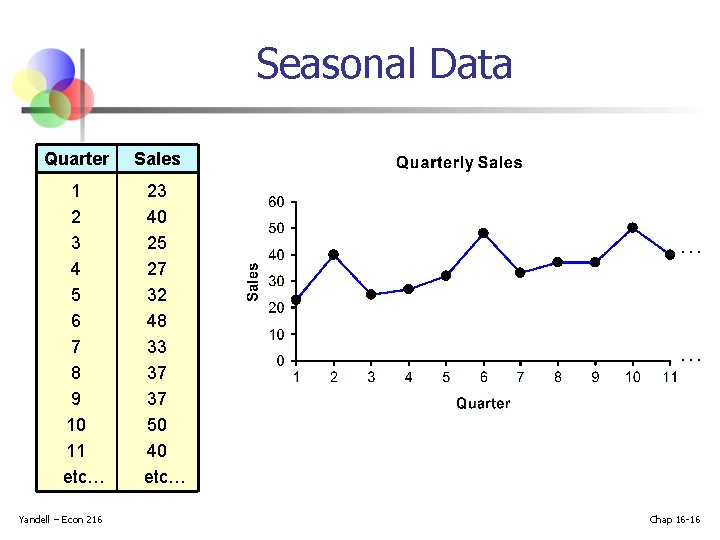
Seasonal Data Quarter Sales 1 2 3 4 5 6 7 8 9 10 11 etc… 23 40 25 27 32 48 33 37 37 50 40 etc… Yandell – Econ 216 … … Chap 16 -16

Calculating Moving Averages Average Period 4 -Quarter Moving Average 23 2. 5 28. 75 2 40 3. 5 31. 00 3 25 4. 5 33. 00 4 27 5. 5 35. 00 5 32 6. 5 37. 50 6 48 7. 5 38. 75 7 33 8. 5 39. 25 8 37 9. 5 41. 00 9 37 10 50 11 40 Quarter Sales 1 Yandell – Econ 216 etc… n Each moving average is for a consecutive block of 4 quarters Chap 16 -17

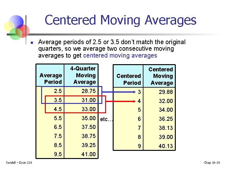
Centered Moving Averages n Yandell – Econ 216 Average periods of 2. 5 or 3. 5 don’t match the original quarters, so we average two consecutive moving averages to get centered moving averages Average Period 4 -Quarter Moving Average Centered Period Centered Moving Average 2. 5 28. 75 3 29. 88 3. 5 31. 00 4 32. 00 4. 5 33. 00 5 34. 00 5. 5 6 36. 25 6. 5 35. 00 etc… 37. 50 7 38. 13 7. 5 38. 75 8 39. 00 8. 5 39. 25 9 40. 13 9. 5 41. 00 Chap 16 -18

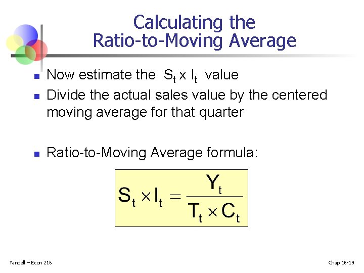
Calculating the Ratio-to-Moving Average n Now estimate the St x It value Divide the actual sales value by the centered moving average for that quarter n Ratio-to-Moving Average formula: n Yandell – Econ 216 Chap 16 -19

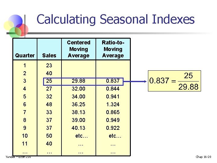
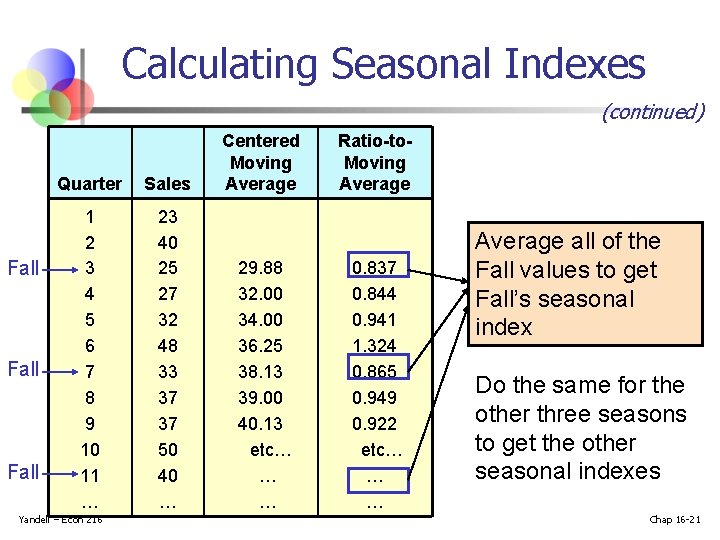
Calculating Seasonal Indexes Quarter Sales Centered Moving Average 1 2 3 4 5 6 7 8 9 10 11 … 23 40 25 27 32 48 33 37 37 50 40 … 29. 88 32. 00 34. 00 36. 25 38. 13 39. 00 40. 13 etc… … … Yandell – Econ 216 Ratio-to. Moving Average 0. 837 0. 844 0. 941 1. 324 0. 865 0. 949 0. 922 etc… … … Chap 16 -20

Calculating Seasonal Indexes (continued) Fall Quarter Sales 1 2 3 4 5 6 7 8 9 10 11 … 23 40 25 27 32 48 33 37 37 50 40 … Yandell – Econ 216 Centered Moving Average 29. 88 32. 00 34. 00 36. 25 38. 13 39. 00 40. 13 etc… … … Ratio-to. Moving Average 0. 837 0. 844 0. 941 1. 324 0. 865 0. 949 0. 922 etc… … … Average all of the Fall values to get Fall’s seasonal index Do the same for the other three seasons to get the other seasonal indexes Chap 16 -21

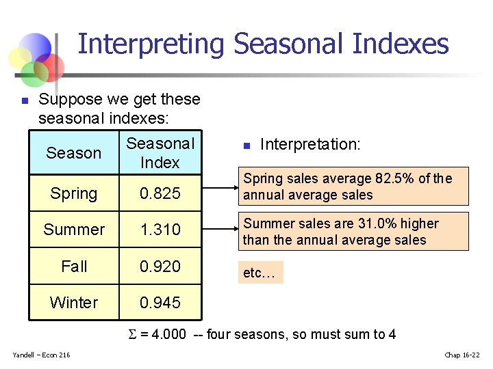
Interpreting Seasonal Indexes n Suppose we get these seasonal indexes: Seasonal Index n Interpretation: Spring 0. 825 Spring sales average 82. 5% of the annual average sales Summer 1. 310 Summer sales are 31. 0% higher than the annual average sales Fall 0. 920 etc… Winter 0. 945 = 4. 000 -- four seasons, so must sum to 4 Yandell – Econ 216 Chap 16 -22

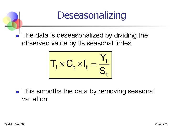
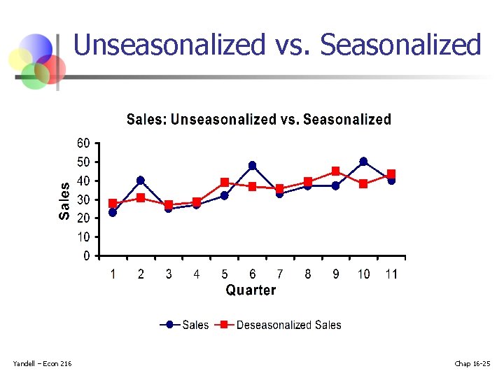
Deseasonalizing n n The data is deseasonalized by dividing the observed value by its seasonal index This smooths the data by removing seasonal variation Yandell – Econ 216 Chap 16 -23

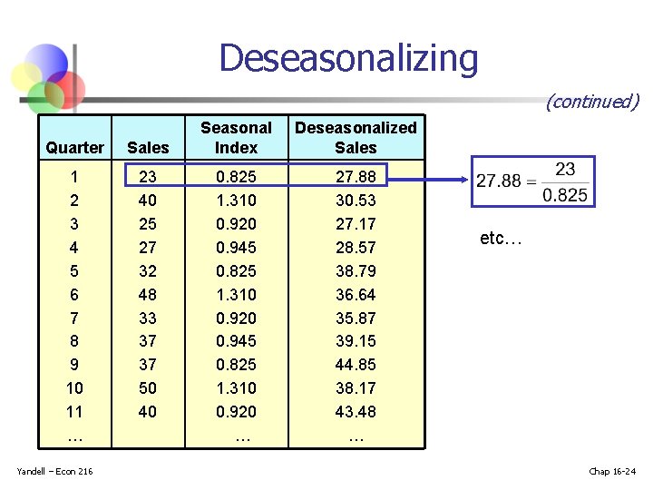
Deseasonalizing (continued) Quarter Sales 1 2 3 4 5 6 7 8 9 10 11 … 23 40 25 27 32 48 33 37 37 50 40 Yandell – Econ 216 Seasonal Index Deseasonalized Sales 0. 825 1. 310 0. 920 0. 945 0. 825 1. 310 0. 920 … 27. 88 30. 53 27. 17 28. 57 38. 79 36. 64 35. 87 39. 15 44. 85 38. 17 43. 48 … etc… Chap 16 -24

Unseasonalized vs. Seasonalized Yandell – Econ 216 Chap 16 -25

Exponential Smoothing n n Yandell – Econ 216 A weighted moving average n Weights decline exponentially n Most recent observation weighted most Used for smoothing and short term forecasting Chap 16 -26

Exponential Smoothing (continued) n The weighting factor is W n n The weight is: n n Yandell – Econ 216 Subjectively chosen Range from 0 to 1 Smaller W gives more smoothing, larger W gives less smoothing Close to 0 for smoothing out unwanted cyclical and irregular components Close to 1 forecasting Chap 16 -27

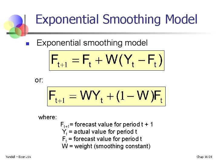
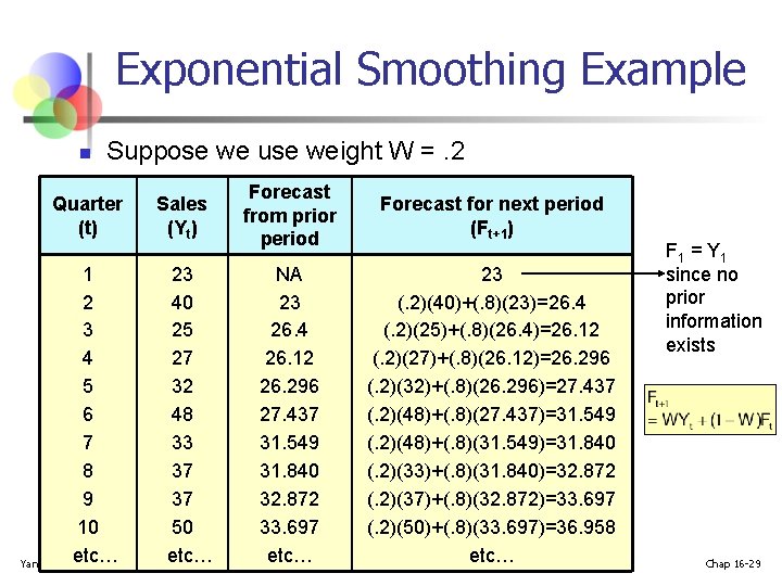
Exponential Smoothing Model n Exponential smoothing model or: where: Ft+1= forecast value for period t + 1 Yt = actual value for period t Ft = forecast value for period t W = weight (smoothing constant) Yandell – Econ 216 Chap 16 -28

Exponential Smoothing Example n Suppose we use weight W =. 2 Quarter (t) 1 2 3 4 5 6 7 8 9 10 etc… Yandell – Econ 216 Sales (Yt) 23 40 25 27 32 48 33 37 37 50 etc… Forecast from prior period Forecast for next period (Ft+1) NA 23 26. 4 26. 12 26. 296 27. 437 31. 549 31. 840 32. 872 33. 697 etc… 23 (. 2)(40)+(. 8)(23)=26. 4 (. 2)(25)+(. 8)(26. 4)=26. 12 (. 2)(27)+(. 8)(26. 12)=26. 296 (. 2)(32)+(. 8)(26. 296)=27. 437 (. 2)(48)+(. 8)(27. 437)=31. 549 (. 2)(48)+(. 8)(31. 549)=31. 840 (. 2)(33)+(. 8)(31. 840)=32. 872 (. 2)(37)+(. 8)(32. 872)=33. 697 (. 2)(50)+(. 8)(33. 697)=36. 958 etc… F 1 = Y 1 since no prior information exists Chap 16 -29

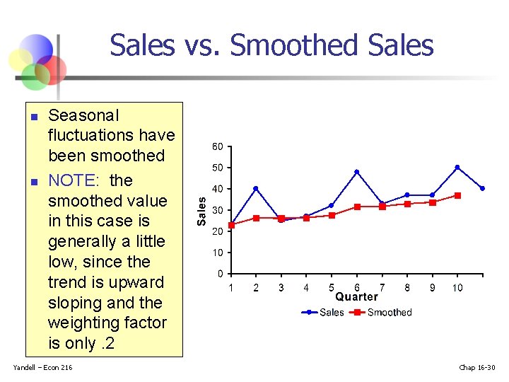
Sales vs. Smoothed Sales n n Seasonal fluctuations have been smoothed NOTE: the smoothed value in this case is generally a little low, since the trend is upward sloping and the weighting factor is only. 2 Yandell – Econ 216 Chap 16 -30

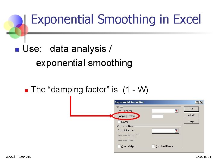
Exponential Smoothing in Excel n Use: data analysis / exponential smoothing n Yandell – Econ 216 The “damping factor” is (1 - W) Chap 16 -31

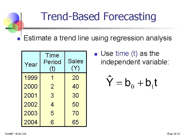
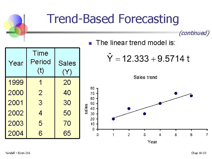
Trend-Based Forecasting n Estimate a trend line using regression analysis Year 1999 2000 2001 2002 2003 2004 Yandell – Econ 216 Time Period (t) 1 2 3 4 5 6 n Sales (Y) Use time (t) as the independent variable: 20 40 30 50 70 65 Chap 16 -32

Trend-Based Forecasting (continued) n Time Year Period (t) 1999 2000 2001 2002 2003 2004 Yandell – Econ 216 1 2 3 4 5 6 The linear trend model is: Sales (Y) 20 40 30 50 70 65 Chap 16 -33

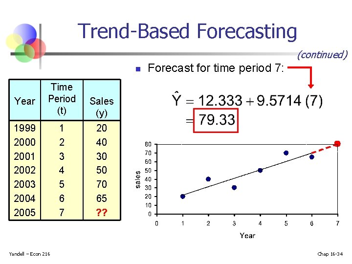
Trend-Based Forecasting (continued) n Year Time Period (t) Sales (y) 1999 2000 2001 2002 2003 2004 2005 1 2 3 4 5 6 7 20 40 30 50 70 65 ? ? Yandell – Econ 216 Forecast for time period 7: Chap 16 -34

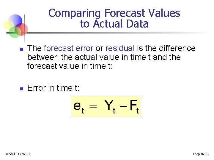
Comparing Forecast Values to Actual Data n n The forecast error or residual is the difference between the actual value in time t and the forecast value in time t: Error in time t: Yandell – Econ 216 Chap 16 -35

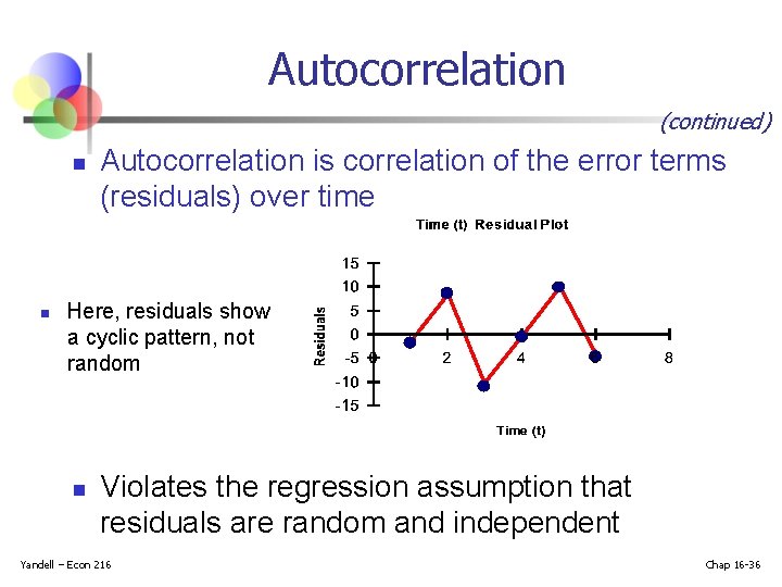
Autocorrelation (continued) n n Autocorrelation is correlation of the error terms (residuals) over time Here, residuals show a cyclic pattern, not random n Violates the regression assumption that residuals are random and independent Yandell – Econ 216 Chap 16 -36

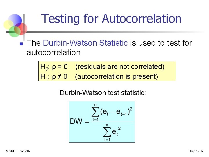
Testing for Autocorrelation n The Durbin-Watson Statistic is used to test for autocorrelation H 0: ρ = 0 H 1: ρ ≠ 0 (residuals are not correlated) (autocorrelation is present) Durbin-Watson test statistic: Yandell – Econ 216 Chap 16 -37

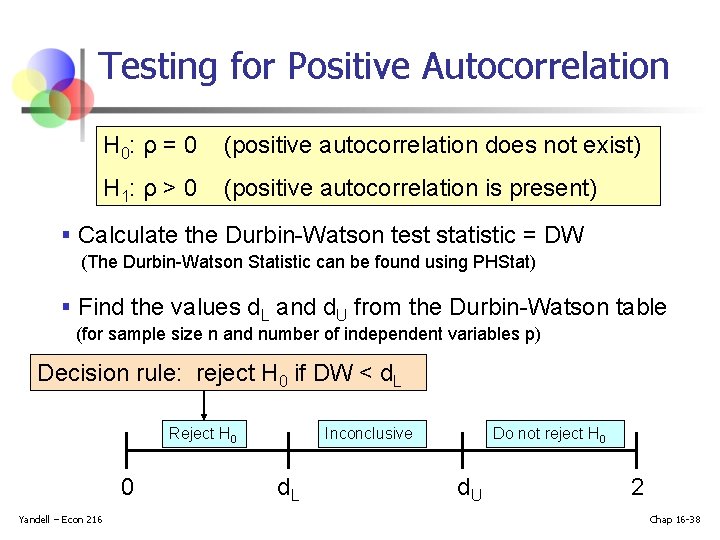
Testing for Positive Autocorrelation H 0: ρ = 0 (positive autocorrelation does not exist) H 1: ρ > 0 (positive autocorrelation is present) § Calculate the Durbin-Watson test statistic = DW (The Durbin-Watson Statistic can be found using PHStat) § Find the values d. L and d. U from the Durbin-Watson table (for sample size n and number of independent variables p) Decision rule: reject H 0 if DW < d. L Reject H 0 0 Yandell – Econ 216 Inconclusive d. L Do not reject H 0 d. U 2 Chap 16 -38

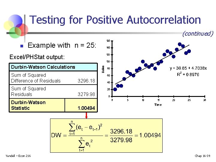
Testing for Positive Autocorrelation (continued) n Example with n = 25: Excel/PHStat output: Durbin-Watson Calculations Sum of Squared Difference of Residuals 3296. 18 Sum of Squared Residuals 3279. 98 Durbin-Watson Statistic 1. 00494 Yandell – Econ 216 Chap 16 -39

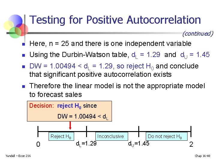
Testing for Positive Autocorrelation (continued) n Here, n = 25 and there is one independent variable n Using the Durbin-Watson table, d. L = 1. 29 and d. U = 1. 45 n n DW = 1. 00494 < d. L = 1. 29, so reject H 0 and conclude that significant positive autocorrelation exists Therefore the linear model is not the appropriate model to forecast sales Decision: reject H 0 since DW = 1. 00494 < d. L Reject H 0 0 Yandell – Econ 216 Inconclusive d. L=1. 29 Do not reject H 0 d. U=1. 45 2 Chap 16 -40

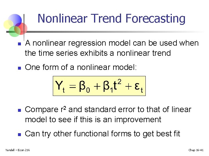
Nonlinear Trend Forecasting n n A nonlinear regression model can be used when the time series exhibits a nonlinear trend One form of a nonlinear model: Compare r 2 and standard error to that of linear model to see if this is an improvement Can try other functional forms to get best fit Yandell – Econ 216 Chap 16 -41

Chapter Summary n n Discussed the importance of forecasting Addressed component factors present in the time-series model Computed and interpreted index numbers Described least square trend fitting and forecasting n n linear and nonlinear models Performed smoothing of data series n n Yandell – Econ 216 moving averages single and double exponential smoothing Chap 16 -42