Chapter 14 Analysis of Variance ANOVA 14 3

14 -3 Two-Way Analysis of Variance • In doing a study that involves a

Assumptions for Two-Way ANOVA 1. The populations from which the samples were obtained must

A company sells three items: Swimming pools, spas, and saunas. The owner decides to

Hypothesis Test A few differences in the 5 step process compared to the two-way

Difference in the means between ROW Headings Step 1: State the hypotheses. Age of

Difference in the means between COLUMN Headings Step 1: State the hypotheses. Age of

Interaction between ROW Headings and COLUMN Headings Step 1: State the hypotheses. Age of

EXCEL will calculate the Critical Value and Test Value In order to use Excel’s

Type the Data with Row headings and Column headings Over 30 30 or under

Highlight the data (including labels) and select Data Analysis on the top ribbon of

Input the entire table 5 Rows per sample --Count the samples for each. In

5 Check OUTPUT RANGE then select which cell to display the results. THEN CLICK

Anova: Two-Factor With Replication SUMMARY Pool Spa Sauna Over 30 5 194 38. 8

ANOVA Source of Variation SS df MS F P-value F crit Sample 168. 0333

To summarize our results, Simply rewrite your hypotheses according to your decisions. Not Rejected

Step 5: Summarize the results. There is no difference among the mean sales between

Example: Gasoline Consumption A researcher wishes to see whether the type of gasoline used

Example: Gasoline Consumption Step 0: Assumptions Step 1: State the hypotheses. The hypotheses for

Example: Gasoline Consumption 1. Input the table information into Excel and request the Two-Way

Example: Gasoline Consumption Two-Way ANOVA Summary Table: ANOVA Source of Variation SS df MS

H 0: There is no difference in mean gas mileage with respect to type

Important note about formatting the data for Excel: Excel will not understand the commas

Slides: 23

Download presentation

Chapter 14: Analysis of Variance (ANOVA) 14 -3 Two-Way Analysis of Variance: Using the two-way ANOVA technique to determine if there is a significant difference in the main effects or interaction.

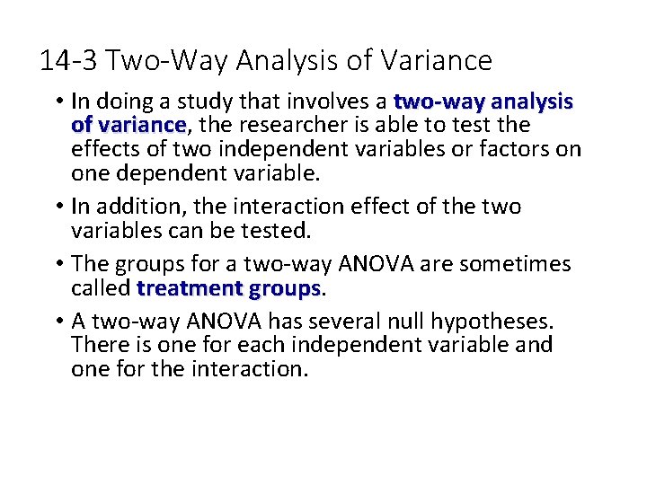
14 -3 Two-Way Analysis of Variance • In doing a study that involves a two-way analysis of variance, the researcher is able to test the variance effects of two independent variables or factors on one dependent variable. • In addition, the interaction effect of the two variables can be tested. • The groups for a two-way ANOVA are sometimes called treatment groups • A two-way ANOVA has several null hypotheses. There is one for each independent variable and one for the interaction.

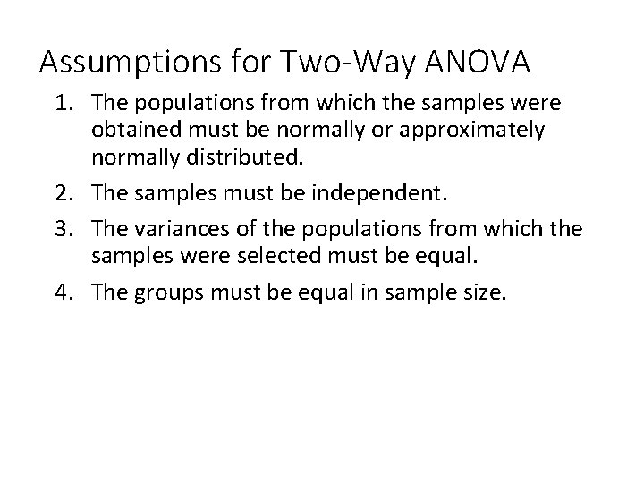
Assumptions for Two-Way ANOVA 1. The populations from which the samples were obtained must be normally or approximately normally distributed. 2. The samples must be independent. 3. The variances of the populations from which the samples were selected must be equal. 4. The groups must be equal in sample size.

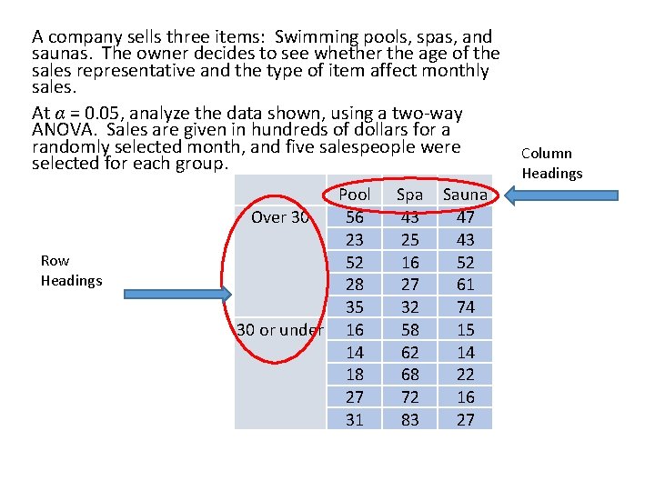
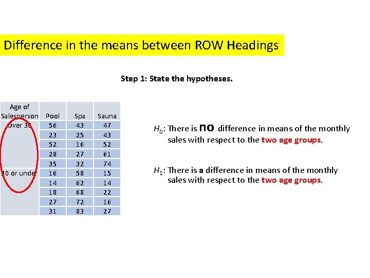
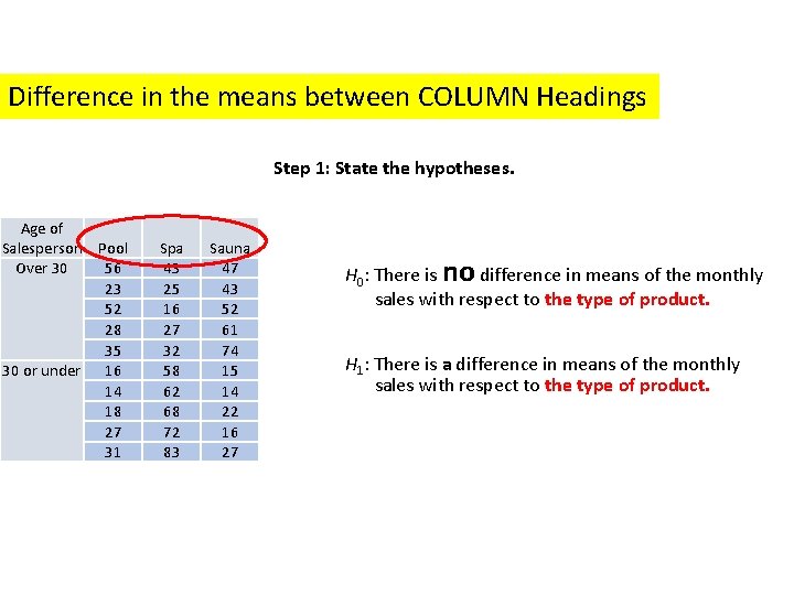
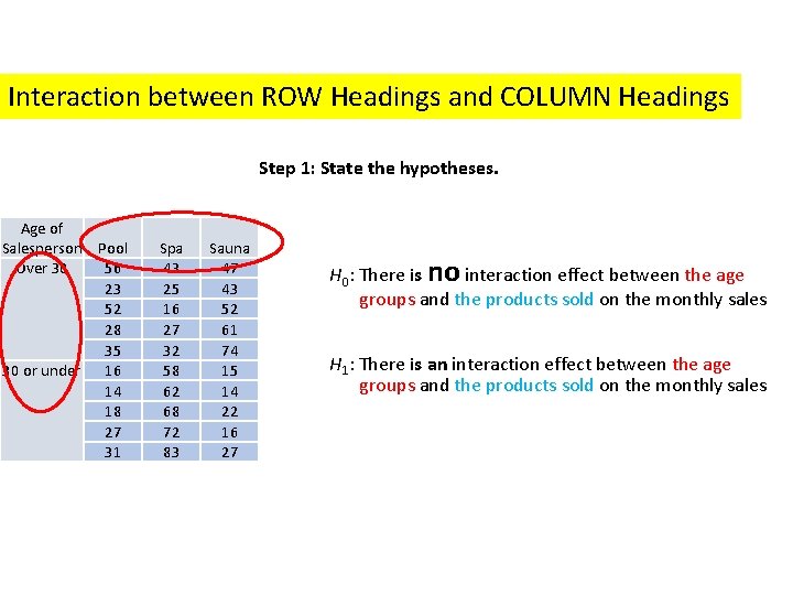
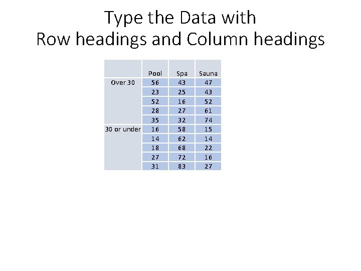
A company sells three items: Swimming pools, spas, and saunas. The owner decides to see whether the age of the sales representative and the type of item affect monthly sales. At α = 0. 05, analyze the data shown, using a two-way ANOVA. Sales are given in hundreds of dollars for a randomly selected month, and five salespeople were Column selected for each group. Headings Row Headings Pool Over 30 56 23 52 28 35 30 or under 16 14 18 27 31 Spa 43 25 16 27 32 58 62 68 72 83 Sauna 47 43 52 61 74 15 14 22 16 27

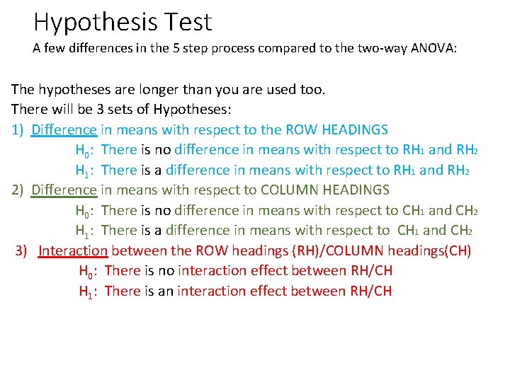
Hypothesis Test A few differences in the 5 step process compared to the two-way ANOVA: The hypotheses are longer than you are used too. There will be 3 sets of Hypotheses: 1) Difference in means with respect to the ROW HEADINGS H 0: There is no difference in means with respect to RH 1 and RH 2 H 1: There is a difference in means with respect to RH 1 and RH 2 2) Difference in means with respect to COLUMN HEADINGS H 0: There is no difference in means with respect to CH 1 and CH 2 H 1: There is a difference in means with respect to CH 1 and CH 2 3) Interaction between the ROW headings (RH)/COLUMN headings(CH) H 0: There is no interaction effect between RH/CH H 1: There is an interaction effect between RH/CH

Difference in the means between ROW Headings Step 1: State the hypotheses. Age of Salesperson Pool Over 30 56 23 52 28 35 30 or under 16 14 18 27 31 Spa 43 25 16 27 32 58 62 68 72 83 Sauna 47 43 52 61 74 15 14 22 16 27 H 0: There is no difference in means of the monthly sales with respect to the two age groups. H 1: There is a difference in means of the monthly sales with respect to the two age groups.

Difference in the means between COLUMN Headings Step 1: State the hypotheses. Age of Salesperson Pool Over 30 56 23 52 28 35 30 or under 16 14 18 27 31 Spa 43 25 16 27 32 58 62 68 72 83 Sauna 47 43 52 61 74 15 14 22 16 27 H 0: There is no difference in means of the monthly sales with respect to the type of product. H 1: There is a difference in means of the monthly sales with respect to the type of product.

Interaction between ROW Headings and COLUMN Headings Step 1: State the hypotheses. Age of Salesperson Pool Over 30 56 23 52 28 35 30 or under 16 14 18 27 31 Spa 43 25 16 27 32 58 62 68 72 83 Sauna 47 43 52 61 74 15 14 22 16 27 H 0: There is no interaction effect between the age groups and the products sold on the monthly sales H 1: There is an interaction effect between the age groups and the products sold on the monthly sales

EXCEL will calculate the Critical Value and Test Value In order to use Excel’s statistics package, we must add it. Follow the instructions provided.

Type the Data with Row headings and Column headings Over 30 30 or under Pool 56 23 52 28 35 16 14 18 27 31 Spa 43 25 16 27 32 58 62 68 72 83 Sauna 47 43 52 61 74 15 14 22 16 27

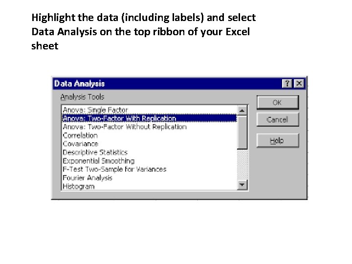
Highlight the data (including labels) and select Data Analysis on the top ribbon of your Excel sheet

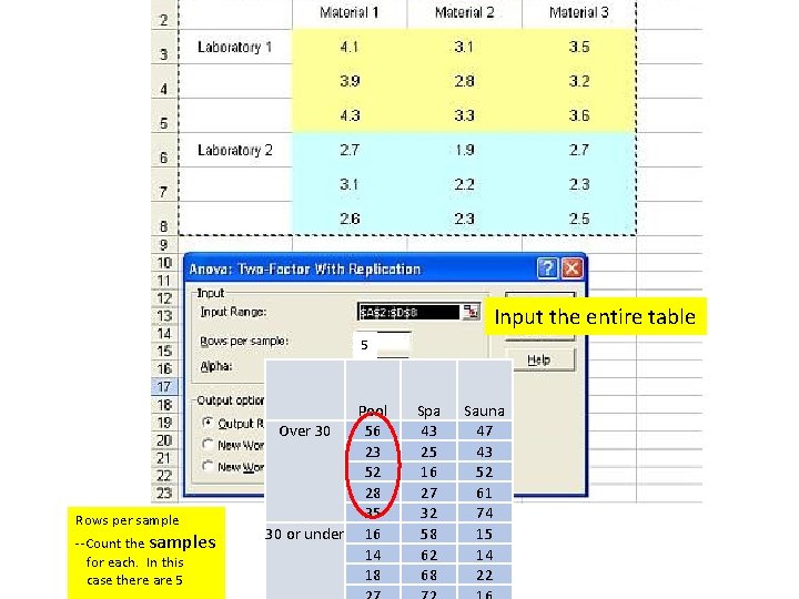
Input the entire table 5 Rows per sample --Count the samples for each. In this case there are 5 Pool Over 30 56 23 52 28 35 30 or under 16 14 18 Spa 43 25 16 27 32 58 62 68 Sauna 47 43 52 61 74 15 14 22

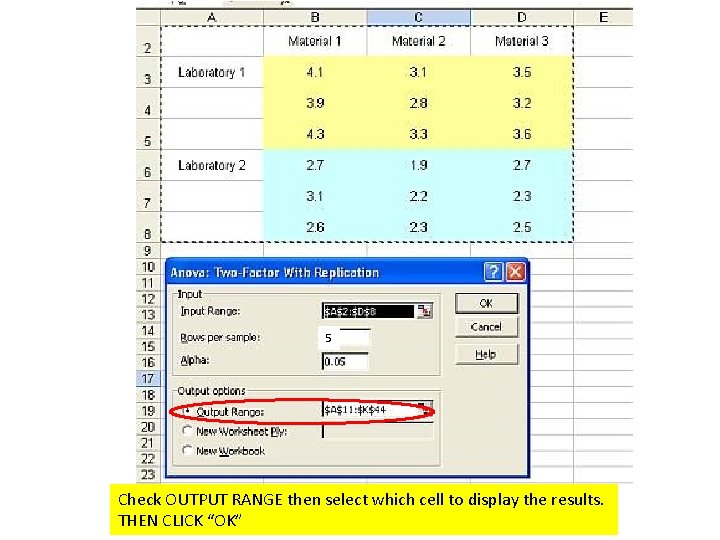
5 Check OUTPUT RANGE then select which cell to display the results. THEN CLICK “OK”

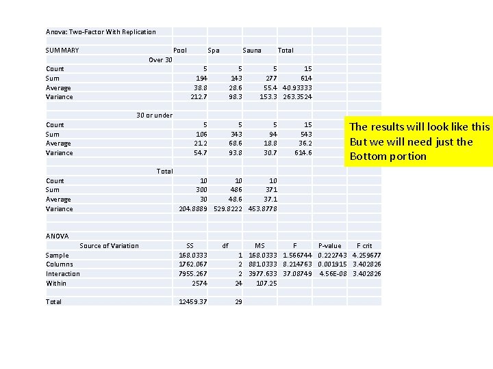
Anova: Two-Factor With Replication SUMMARY Pool Spa Sauna Over 30 5 194 38. 8 212. 7 5 143 28. 6 98. 3 30 or under 5 106 21. 2 54. 7 5 343 68. 6 93. 8 Count Sum Average Variance Total 5 15 277 614 55. 4 40. 93333 153. 3 263. 3524 5 94 18. 8 30. 7 15 543 36. 2 614. 6 The results will look like this But we will need just the Bottom portion 10 10 10 300 486 371 30 48. 6 37. 1 204. 8889 529. 8222 453. 8778 ANOVA Source of Variation Sample Columns Interaction Within SS 168. 0333 1762. 067 7955. 267 2574 Total 12459. 37 df 1 2 2 24 29 MS F P-value F crit 168. 0333 1. 566744 0. 222743 4. 259677 881. 0333 8. 214763 0. 001915 3. 402826 3977. 633 37. 08749 4. 56 E-08 3. 402826 107. 25

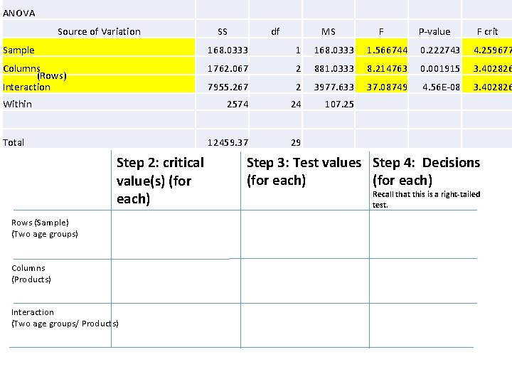
ANOVA Source of Variation SS df MS F P-value F crit Sample 168. 0333 1. 566744 0. 222743 4. 259677 Columns (Rows) Interaction 1762. 067 2 881. 0333 8. 214763 0. 001915 3. 402826 7955. 267 2 3977. 633 37. 08749 4. 56 E-08 3. 402826 2574 24 107. 25 Within Total 12459. 37 Step 2: critical value(s) (for each) Rows (Sample) (Two age groups) Columns (Products) Interaction (Two age groups/ Products) 29 Step 3: Test values Step 4: Decisions (for each) Recall that this is a right-tailed test.

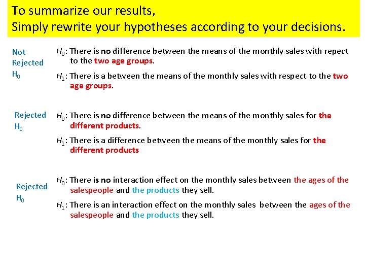
To summarize our results, Simply rewrite your hypotheses according to your decisions. Not Rejected H 0: There is no difference between the means of the monthly sales with repect to the two age groups. H 1: There is a between the means of the monthly sales with respect to the two age groups. Rejected H 0: There is no difference between the means of the monthly sales for the different products. H 0 H 1: There is a difference between the means of the monthly sales for the different products Rejected H 0: There is no interaction effect on the monthly sales between the ages of the salespeople and the products they sell. H 1: There is an interaction effect on the monthly sales between the ages of the salespeople and the products they sell.

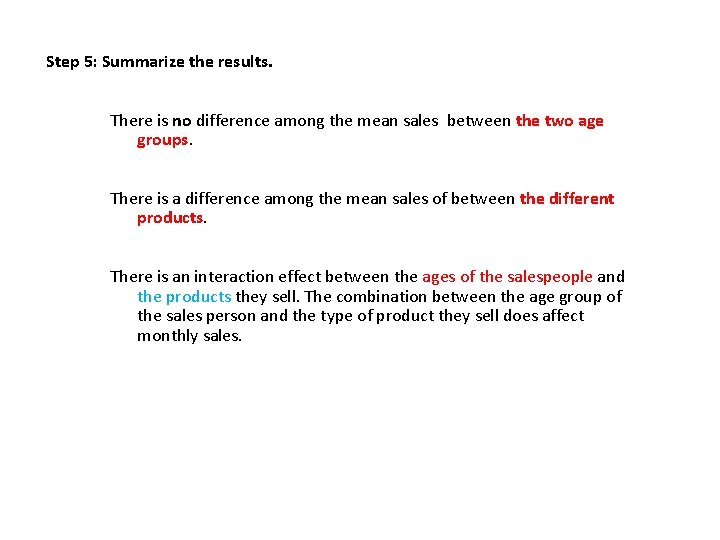
Step 5: Summarize the results. There is no difference among the mean sales between the two age groups. There is a difference among the mean sales of between the different products. There is an interaction effect between the ages of the salespeople and the products they sell. The combination between the age group of the sales person and the type of product they sell does affect monthly sales.

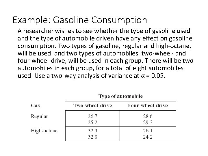
Example: Gasoline Consumption A researcher wishes to see whether the type of gasoline used and the type of automobile driven have any effect on gasoline consumption. Two types of gasoline, regular and high-octane, will be used, and two types of automobiles, two-wheel- and four-wheel-drive, will be used in each group. There will be two automobiles in each group, for a total of eight automobiles used. Use a two-way analysis of variance at α = 0. 05.

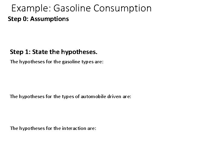
Example: Gasoline Consumption Step 0: Assumptions Step 1: State the hypotheses. The hypotheses for the gasoline types are: The hypotheses for the types of automobile driven are: The hypotheses for the interaction are:

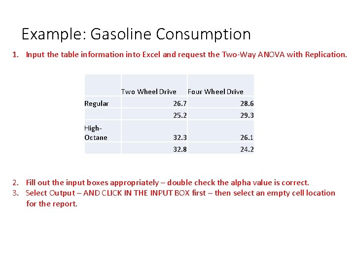
Example: Gasoline Consumption 1. Input the table information into Excel and request the Two-Way ANOVA with Replication. Two Wheel Drive Regular High. Octane Four Wheel Drive 26. 7 28. 6 25. 2 29. 3 32. 3 26. 1 32. 8 24. 2 2. Fill out the input boxes appropriately – double check the alpha value is correct. 3. Select Output – AND CLICK IN THE INPUT BOX first – then select an empty cell location for the report.

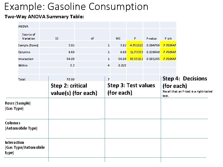
Example: Gasoline Consumption Two-Way ANOVA Summary Table: ANOVA Source of Variation SS df MS F P-value F crit Sample (Rows) 3. 92 1 3. 92 4. 751515 0. 094766 7. 708647 Columns 9. 68 11. 73333 0. 026648 7. 708647 54. 08 1 54. 08 65. 55152 0. 001265 7. 708647 3. 3 4 0. 825 Interaction Within Total 70. 98 Step 2: critical value(s) (for each) Rows (Sample) (Gas Type) Columns (Automobile Type) Interaction (Gas Type/Automobile type) 7 Step 3: Test values (for each) Step 4: Decisions (for each) Recall that an F-test is a right-tailed test.

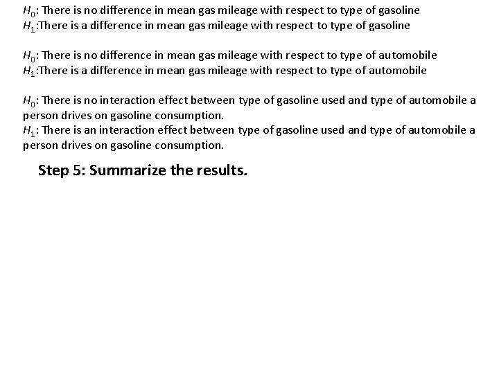
H 0: There is no difference in mean gas mileage with respect to type of gasoline H 1: There is a difference in mean gas mileage with respect to type of gasoline H 0: There is no difference in mean gas mileage with respect to type of automobile H 1: There is a difference in mean gas mileage with respect to type of automobile H 0: There is no interaction effect between type of gasoline used and type of automobile a person drives on gasoline consumption. H 1: There is an interaction effect between type of gasoline used and type of automobile a person drives on gasoline consumption. Step 5: Summarize the results.

Important note about formatting the data for Excel: Excel will not understand the commas between the numbers. For the above data set – your data values must be separated into their own rows:

Related presentations