Chapter 11 Kriging is a spatial prediction method

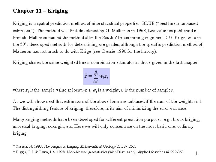
Chapter 11 – Kriging is a spatial prediction method of nice statistical properties: BLUE (“best linear unbiased estimator”). The method was first developed by G. Matheron in 1963, two volumes published in French. Matheron named the method after the South African mining engineer, D. G. Krige, who in the 50’s developed methods for determining ore grades, although the specific prediction method of Matheron has not much to do with Krige (see Cressie 1990 for the history). Kriging shares the same weighted linear combination estimator as those given in the last chapter: where zi is the sample value at location i, wi is a weight, n is the number of samples. As we will show next that estimators of the above form are unbiased if the sum of the weights is 1. The distinguishing feature of kriging, therefore, is its aim of minimizing the error variance. Many kriging methods have been developed for different prediction purposes, e. g. , block kriging, universal kriging, cokrigin, etc. Here we will only concentrate on the most basic one: ordinary kriging. * Cressie, N. 1990. The origins of kriging. Mathematical Geology 22: 239 -252. * Diggle, P. J. & Tawn, J. A. 1998. Model-based geostatistics (with Discussion). Applied Statistics 47: 299 -350. 1

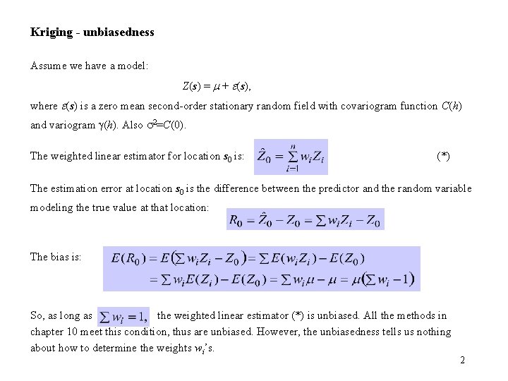
Kriging - unbiasedness Assume we have a model: Z(s) = m + (s), where (s) is a zero mean second-order stationary random field with covariogram function C(h) and variogram g(h). Also 2=C(0). The weighted linear estimator for location s 0 is: (*) The estimation error at location s 0 is the difference between the predictor and the random variable modeling the true value at that location: The bias is: So, as long as the weighted linear estimator (*) is unbiased. All the methods in chapter 10 meet this condition, thus are unbiased. However, the unbiasedness tells us nothing about how to determine the weights wi’s. 2

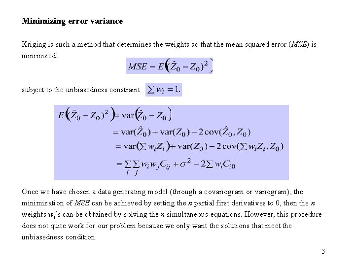
Minimizing error variance Kriging is such a method that determines the weights so that the mean squared error (MSE) is minimized: subject to the unbiasedness constraint Once we have chosen a data generating model (through a covariogram or variogram), the minimization of MSE can be achieved by setting the n partial first derivatives to 0, then the n weights wi’s can be obtained by solving the n simultaneous equations. However, this procedure does not quite work for our problem because we only want the solutions that meet the unbiasedness condition. 3

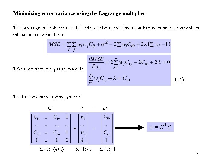
Minimizing error variance using the Lagrange multiplier The Lagrange multiplier is a useful technique for converting a constrained minimization problem into an unconstrained one. Take the first term w 1 as an example: (**) The final ordinary kriging system is: C w = D w = C-1 D (n+1) 1 4

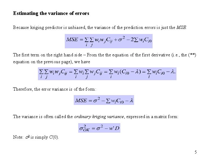
Estimating the variance of errors Because kriging predictor is unbiased, the variance of the prediction errors is just the MSE: The first term on the right hand side – From the equation of the first derivative (i. e. , the (**) equation on the previous page), we have Therefore, the error variance is of the form: The variance is often called the ordinary kriging variance, expressed in a matrix form: Note: s 2 is simply C(0). 5

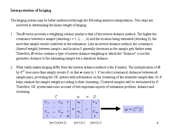
Interpretation of kriging The kriging system may be better understood through the following intuitive interpretation. Two steps are involved in determining the linear weight of kriging: 1. The D vector provides a weighting scheme similar to that of the inverse distance method. The higher the covariance between a sample (denoting i = 1, 2, …, n) and the location being estimated (denoting 0), the more that sample would contribute to the estimation. Like an inverse distance method, the covariance (thereof weight) between sample i and location 0 generally decreases as the sample gets farther away. Therefore, D vector contains a type of inverse distance weighting in which the “distance” is not the geometric distance to the estimating sample but a statistical distance. 2. What really makes kriging differ from the inverse distance method is the C matrix. The multiplication of D by C-1 does more than simply rescale D so that w sums to 1. C records (covariance) distances between all sample pairs, providing the OK system with information on the clustering of the available sample data. So C helps readjust the sample weight according to their clustering. Clustered samples will be declustered by C. Therefore, OK system takes into account of two important aspects of estimation problem: distance and clustering. C w = D w = C-1 D (n+1) 1 6

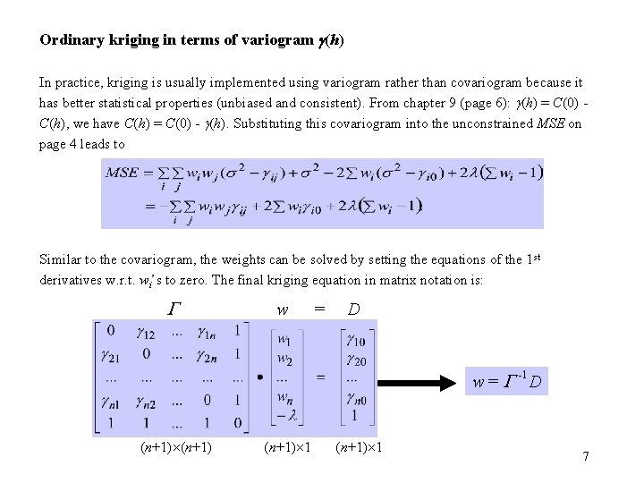
Ordinary kriging in terms of variogram g(h) In practice, kriging is usually implemented using variogram rather than covariogram because it has better statistical properties (unbiased and consistent). From chapter 9 (page 6): g(h) = C(0) - C(h), we have C(h) = C(0) - g(h). Substituting this covariogram into the unconstrained MSE on page 4 leads to Similar to the covariogram, the weights can be solved by setting the equations of the 1 st derivatives w. r. t. wi’s to zero. The final kriging equation in matrix notation is: w = D w = -1 D (n+1) 1 7

Ordinary kriging variance in terms of variogram g(h) Following the same steps as for the variance based on the covariogram, we have the ordinary kriging variance in terms of variogram: where w and D are the vectors given on the previous page. Steps for kriging – 1. 2. 3. 4. 5. 6. 7. EDA exploration, removing trend, checking for stationarity and isotropy Computing the empirical variogram Fitting and selecting a theoretical variogram model to the empirical variogram Computing the weight w using the fitted theoretical variogram, i. e. , kriging. Predicting the values at the locations of interest Validation Plotting kriging surfaces 8

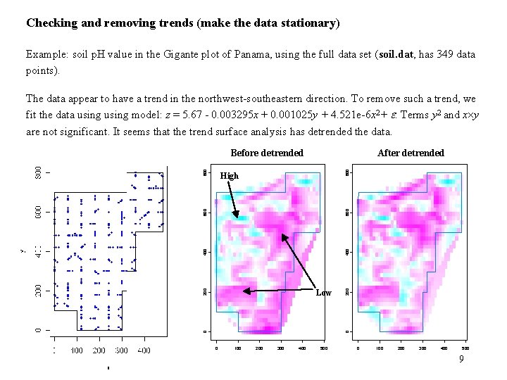
Checking and removing trends (make the data stationary) Example: soil p. H value in the Gigante plot of Panama, using the full data set (soil. dat, has 349 data points). The data appear to have a trend in the northwest-southeastern direction. To remove such a trend, we fit the data using model: z = 5. 67 - 0. 003295 x + 0. 001025 y + 4. 521 e-6 x 2+ . Terms y 2 and x y are not significant. It seems that the trend surface analysis has detrended the data. After detrended 800 Before detrended 0 0 200 Low 200 400 600 High 0 100 200 300 400 500 9

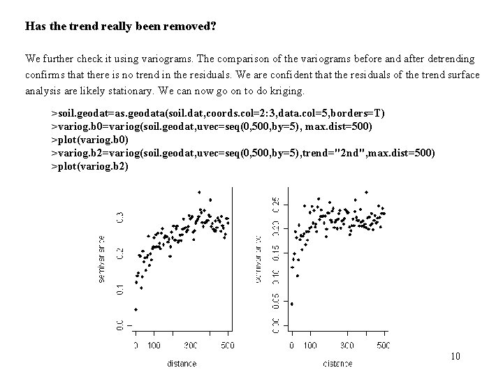
Has the trend really been removed? We further check it using variograms. The comparison of the variograms before and after detrending confirms that there is no trend in the residuals. We are confident that the residuals of the trend surface analysis are likely stationary. We can now go on to do kriging. >soil. geodat=as. geodata(soil. dat, coords. col=2: 3, data. col=5, borders=T) >variog. b 0=variog(soil. geodat, uvec=seq(0, 500, by=5), max. dist=500) >plot(variog. b 0) >variog. b 2=variog(soil. geodat, uvec=seq(0, 500, by=5), trend="2 nd", max. dist=500) >plot(variog. b 2) 10

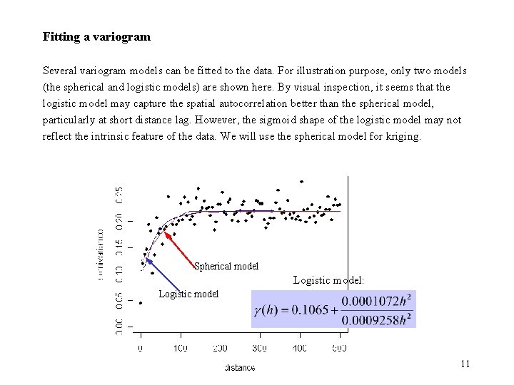
Fitting a variogram Several variogram models can be fitted to the data. For illustration purpose, only two models (the spherical and logistic models) are shown here. By visual inspection, it seems that the logistic model may capture the spatial autocorrelation better than the spherical model, particularly at short distance lag. However, the sigmoid shape of the logistic model may not reflect the intrinsic feature of the data. We will use the spherical model for kriging. Spherical model Logistic model: Logistic model 11

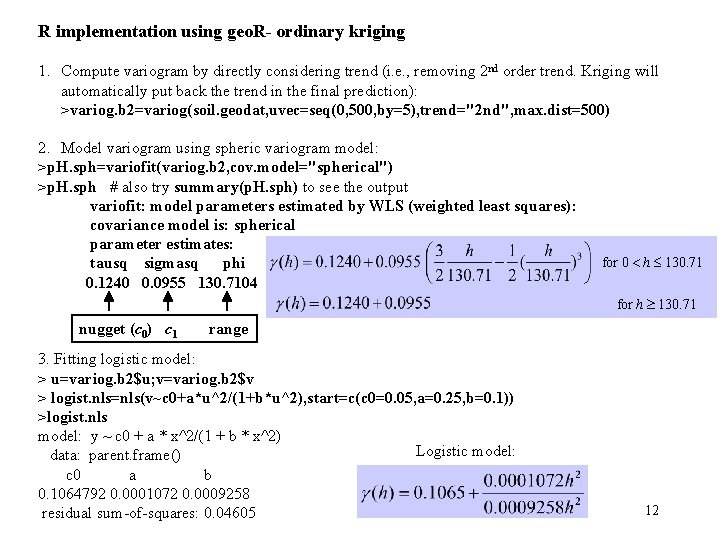
R implementation using geo. R- ordinary kriging 1. Compute variogram by directly considering trend (i. e. , removing 2 nd order trend. Kriging will automatically put back the trend in the final prediction): >variog. b 2=variog(soil. geodat, uvec=seq(0, 500, by=5), trend="2 nd", max. dist=500) 2. Model variogram using spheric variogram model: >p. H. sph=variofit(variog. b 2, cov. model="spherical") >p. H. sph # also try summary(p. H. sph) to see the output variofit: model parameters estimated by WLS (weighted least squares): covariance model is: spherical parameter estimates: tausq sigmasq phi 0. 1240 0. 0955 130. 7104 for 0 h 130. 71 for h 130. 71 nugget (c 0) c 1 range 3. Fitting logistic model: > u=variog. b 2$u; v=variog. b 2$v > logist. nls=nls(v~c 0+a*u^2/(1+b*u^2), start=c(c 0=0. 05, a=0. 25, b=0. 1)) >logist. nls model: y ~ c 0 + a * x^2/(1 + b * x^2) Logistic model: data: parent. frame() c 0 a b 0. 1064792 0. 0001072 0. 0009258 residual sum-of-squares: 0. 04605 12

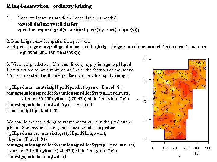
R implementation - ordinary kriging 1. Generate locations at which interpolation is needed: >x=soil. dat$gx; y=soil. dat$gy >prd. loc=expand. grid(x=sort(unique(x)), y=sort(unique(y))) 2. Run krige. conv for spatial interpolation: >p. H. prd=krige. conv(soil. geodat, loc=prd. loc, krige=krige. control(cov. model="spherical", cov. pars =c(0. 09549404, 130. 71043698))) 3. View the prediction: You can directly apply image to p. H. prd. Here we want to have more control over the features of the image, We create matrix for the p. H. prd$predict and then apply image: >p. H. prd. mat=matrix(p. H. prd$predict, byrow=T, ncol=84) >image(unique(prd. loc$x), unique(prd. loc$y), t(p. H. prd. mat), xlim=c(-20, 500), ylim=c(-20, 820), xlab="x", ylab="y") >lines(gigante. border, lwd=2, col=“green”) >contour(p. H. prd, add=T) We can do the same thing to view the variation in the prediction: p. H. prd$krige. var. Taking the squared root, it is prd. se. >p. H. prd. se. mat=matrix(sqrt(p. H. prd$krige. var), byrow=T, ncol=84) >image(unique(prd. loc$x), unique(prd. loc$y), t(p. H. prd. se. mat), xlim=c(-20, 500), ylim=c(-20, 820), xlab="x", ylab="y") >lines(gigante. border, lwd=2) 13

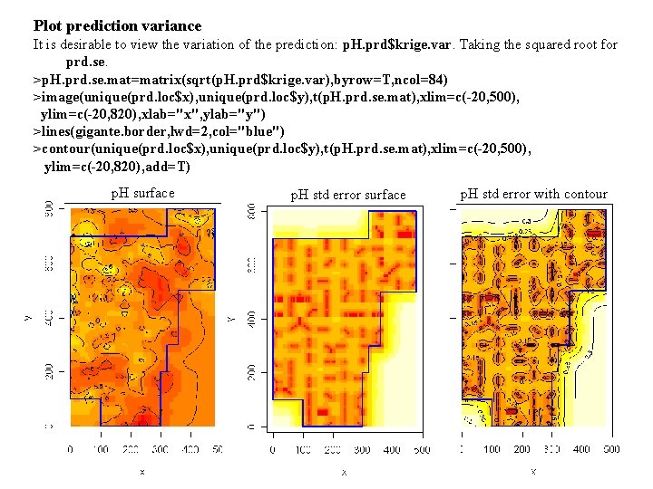
Plot prediction variance It is desirable to view the variation of the prediction: p. H. prd$krige. var. Taking the squared root for prd. se. >p. H. prd. se. mat=matrix(sqrt(p. H. prd$krige. var), byrow=T, ncol=84) >image(unique(prd. loc$x), unique(prd. loc$y), t(p. H. prd. se. mat), xlim=c(-20, 500), ylim=c(-20, 820), xlab="x", ylab="y") >lines(gigante. border, lwd=2, col="blue") >contour(unique(prd. loc$x), unique(prd. loc$y), t(p. H. prd. se. mat), xlim=c(-20, 500), ylim=c(-20, 820), add=T) p. H surface p. H std error with contour 14

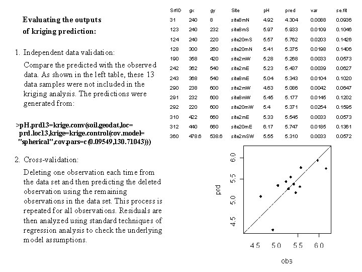
Evaluating the outputs of kriging prediction: 1. Independent data validation: Compare the predicted with the observed data. As shown in the left table, these 13 data samples were not included in the kriging analysis. The predictions were generated from: >p. H. prd 13=krige. conv(soil. geodat, loc= prd. loc 13, krige=krige. control(cov. model= "spherical", cov. pars=c(0. 09549, 130. 71043))) Srf. ID gx gy Site p. H pred var se. fit 31 240 8 site 8 m. N 4. 92 4. 304 0. 0088 0. 0936 123 240 232 site 8 m. S 5. 97 5. 933 0. 0109 0. 1046 124 240 220 site 20 m. S 5. 57 5. 762 0. 0203 0. 1426 128 300 260 site 20 m. N 5. 41 5. 375 0. 0198 0. 1406 190 358 420 site 2 m. W 5. 28 5. 268 0. 0033 0. 0573 242 362 540 site 2 m. E 5. 23 5. 437 0. 0039 0. 0627 243 368 540 site 8 m. E 5. 04 5. 343 0. 0104 0. 1020 290 238 600 site 2 m. W 4. 63 5. 086 0. 0042 0. 0647 291 232 600 site 8 m. W 5. 45 5. 177 0. 0145 0. 1202 292 220 600 site 20 m. W 5. 4 5. 371 0. 0254 0. 1595 310 422 660 site 2 m. E 5. 33 5. 545 0. 0033 0. 0573 312 440 660 site 20 m. E 6. 17 5. 747 0. 0185 0. 1361 360 478. 6 538. 6 site 2 m. SW 5. 55 5. 310 0. 0033 0. 0572 2. Cross-validation: Deleting one observation each time from the data set and then predicting the deleted observation using the remaining observations in the data set. This process is repeated for all observations. Residuals are then analyzed using standard techniques of regression analysis to check the underlying model assumptions. 15

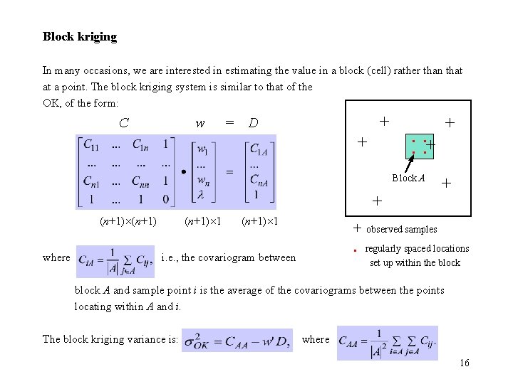
Block kriging In many occasions, we are interested in estimating the value in a block (cell) rather than that at a point. The block kriging system is similar to that of the OK, of the form: C + w = D + . . + Block A + (n+1) 1 where i. e. , the covariogram between + + + observed samples . regularly spaced locations set up within the block A and sample point i is the average of the covariograms between the points locating within A and i. The block kriging variance is: where 16

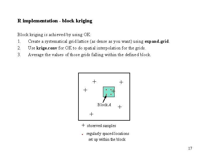
R implementation - block kriging Block kriging is achieved by using OK: 1. Create a systematical grid lattice (as dense as you want) using expand. grid. 2. Use krige. conv for OK to do spatial interpolation for the grids. 3. Average the values of those grids falling within the defined block. + + . . + Block A + + observed samples . regularly spaced locations set up within the block 17

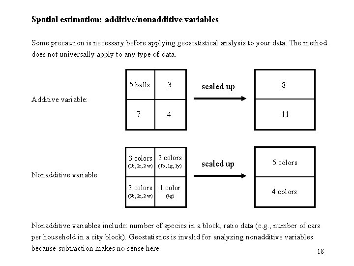
Spatial estimation: additive/nonadditive variables Some precaution is necessary before applying geostatistical analysis to your data. The method does not universally apply to any type of data. 5 balls 3 7 4 scaled up 8 Additive variable: 3 colors (1 b, 2 r, 2 w) (1 b, 1 g, 1 y) 3 colors 1 color (3 b, 2 r, 2 w) (4 g) 11 scaled up 5 colors Nonadditive variable: 4 colors Nonadditive variables include: number of species in a block, ratio data (e. g. , number of cars per household in a city block). Geostatistics is invalid for analyzing nonadditive variables because subtraction makes no sense here. 18

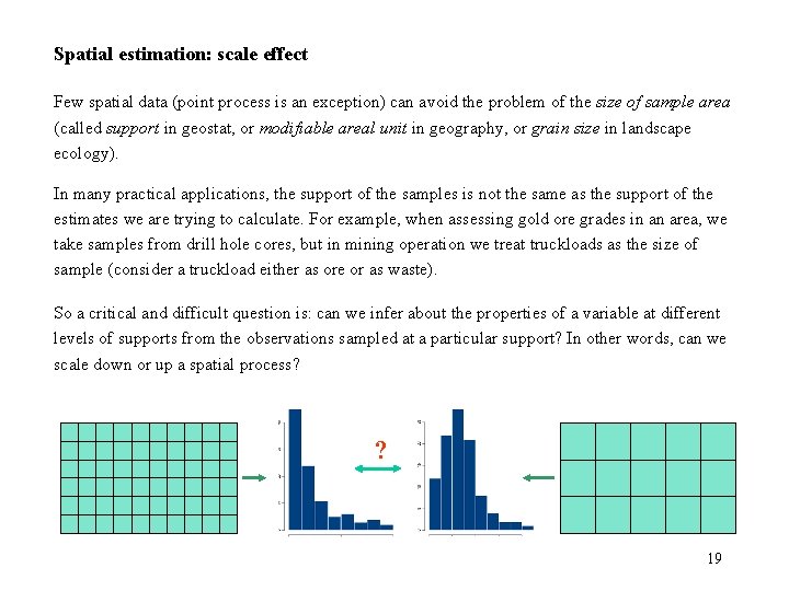
Spatial estimation: scale effect Few spatial data (point process is an exception) can avoid the problem of the size of sample area (called support in geostat, or modifiable areal unit in geography, or grain size in landscape ecology). In many practical applications, the support of the samples is not the same as the support of the estimates we are trying to calculate. For example, when assessing gold ore grades in an area, we take samples from drill hole cores, but in mining operation we treat truckloads as the size of sample (consider a truckload either as ore or as waste). So a critical and difficult question is: can we infer about the properties of a variable at different levels of supports from the observations sampled at a particular support? In other words, can we scale down or up a spatial process? ? 19

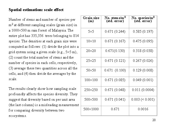
Spatial estimation: scale effect Grain size Number of stems and number of species per (m) 2 m at different sampling scales (grain size) in a 1000 500 m rain forest of Malaysia. The 5 5 entire plot has 335, 356 trees belonging to 814 10 10 species. The densities at each grain size were computed as follows: (1) divide the plot into a 20 20 grid system using a given scale (e. g. , 5 5 m), (2) count the total number of stems and the 25 25 number of species in each cells, respectively, (3) average these two quantities across all the 50 50 cells, and (4) then divide the averages by the scale. 100 The results clearly show sampling scale 250 profoundly affects the species diversity. They suggest that diversity based on per unit area 500 (the last column) is a misleading measurement 500 1000 for comparing diversity between two ecosystems. No. stems/m 2 (std. error) No. species/m 2 (std. error) 0. 671 (0. 244) 0. 585 (0. 197) 0. 671 (0. 167) 0. 475 (0. 095) 0. 671(0. 130) 0. 318 (0. 038) 0. 671 (0. 121) 0. 267 (0. 026) 0. 671 (0. 100) 0. 129 (0. 008) 0. 671 (0. 085) 0. 049 (0. 001) 0. 671 (0. 048) 0. 011 (0. 0004) 0. 671 (0. 041) 0. 003 (< 0. 001) 0. 671 0. 0016 20

Spatial estimation: scale effect “This problem of the discrepancy between the support of our samples and the intended support of our estimates is one of the most difficult we face in estimation. ” Isaaks & Srivastava (1989, page 193) 21