7 Prediction Error Method 1 Prediction Error Consider

(7) Prediction Error Method 1

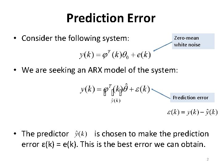
Prediction Error • Consider the following system: Zero-mean white noise • We are seeking an ARX model of the system: Prediction error • The predictor is chosen to make the prediction error ε(k) = e(k). This is the best error we can obtain. 2

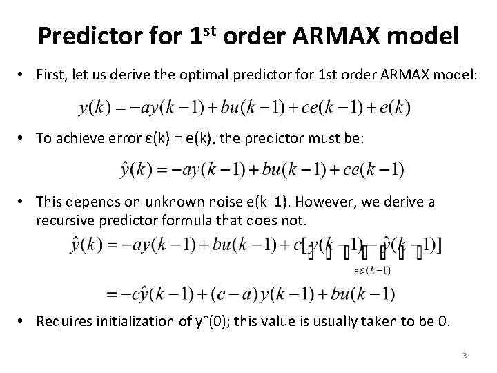
Predictor for 1 st order ARMAX model • First, let us derive the optimal predictor for 1 st order ARMAX model: • To achieve error ε(k) = e(k), the predictor must be: • This depends on unknown noise e(k− 1). However, we derive a recursive predictor formula that does not. • Requires initialization of yᵔ(0); this value is usually taken to be 0. 3

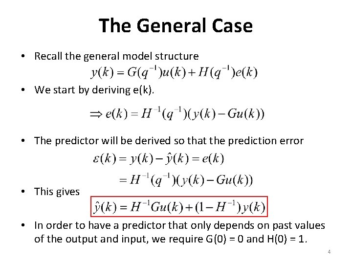
The General Case • Recall the general model structure • We start by deriving e(k). • The predictor will be derived so that the prediction error • This gives • In order to have a predictor that only depends on past values of the output and input, we require G(0) = 0 and H(0) = 1. 4

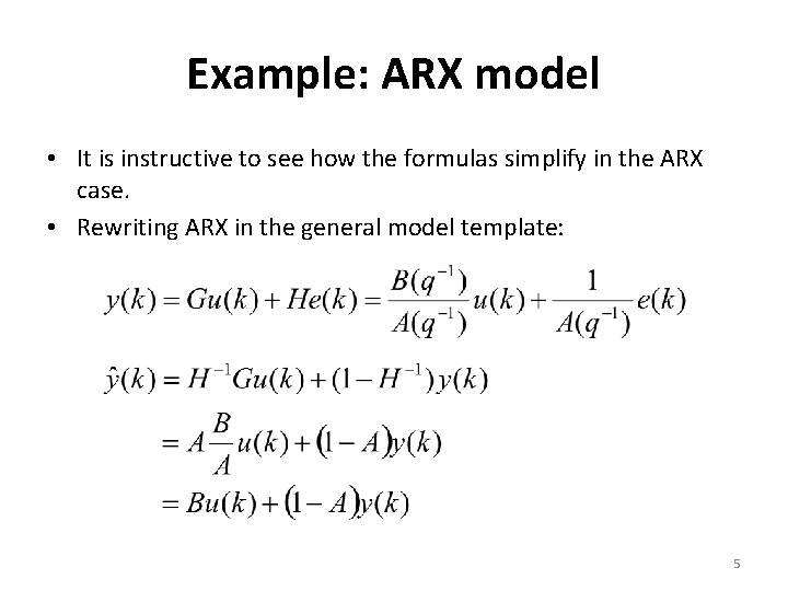
Example: ARX model • It is instructive to see how the formulas simplify in the ARX case. • Rewriting ARX in the general model template: 5

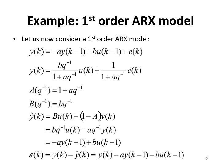
Example: 1 st order ARX model • Let us now consider a 1 st order ARX model: 6

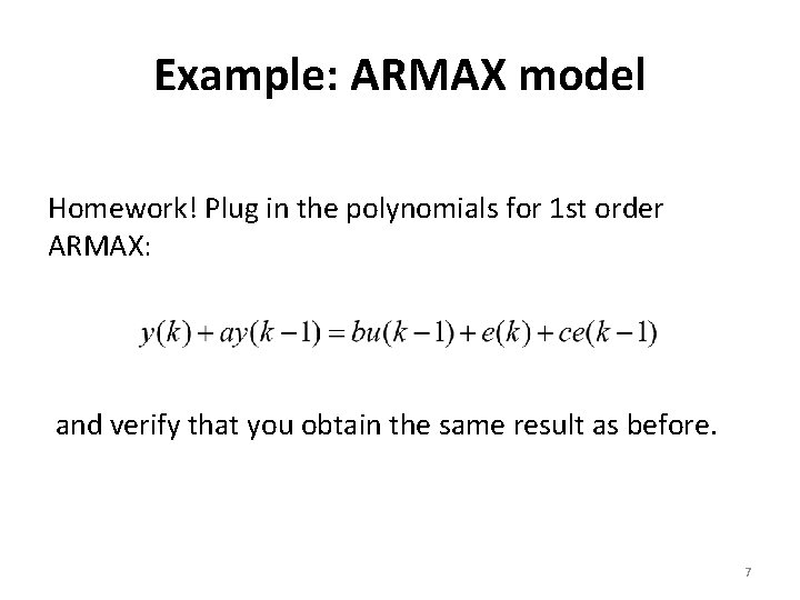
Example: ARMAX model Homework! Plug in the polynomials for 1 st order ARMAX: and verify that you obtain the same result as before. 7

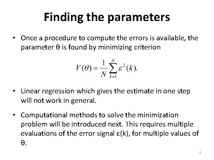
Finding the parameters • Once a procedure to compute the errors is available, the parameter θ is found by minimizing criterion • Linear regression which gives the estimate in one step will not work in general. • Computational methods to solve the minimization problem will be introduced next. This requires multiple evaluations of the error signal ε(k), for multiple values of θ. 8

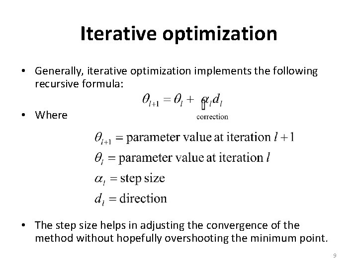
Iterative optimization • Generally, iterative optimization implements the following recursive formula: • Where • The step size helps in adjusting the convergence of the method without hopefully overshooting the minimum point. 9

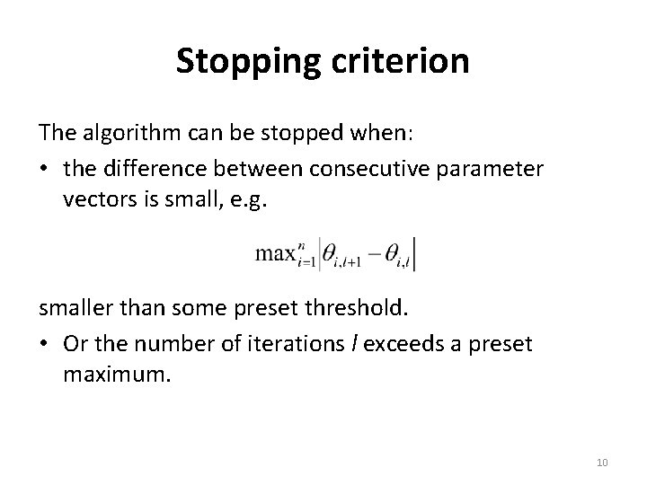
Stopping criterion The algorithm can be stopped when: • the difference between consecutive parameter vectors is small, e. g. smaller than some preset threshold. • Or the number of iterations l exceeds a preset maximum. 10

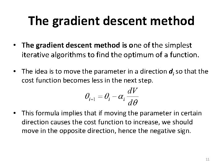
The gradient descent method • The gradient descent method is one of the simplest iterative algorithms to find the optimum of a function. • The idea is to move the parameter in a direction di so that the cost function becomes less in the next step. • This formula implies that if moving the parameter in certain direction causes the cost function to increase, we should move in the opposite direction, hence the negative sign. 11

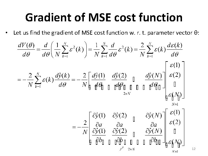
Gradient of MSE cost function • Let us find the gradient of MSE cost function w. r. t. parameter vector θ: 12

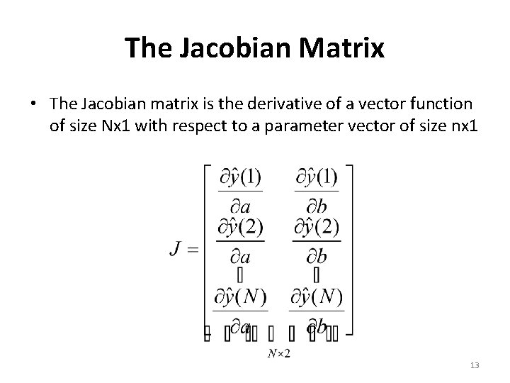
The Jacobian Matrix • The Jacobian matrix is the derivative of a vector function of size Nx 1 with respect to a parameter vector of size nx 1 13

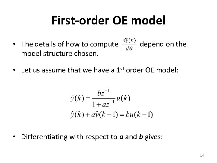
First-order OE model • The details of how to compute model structure chosen. depend on the • Let us assume that we have a 1 st order OE model: • Differentiating with respect to a and b gives: 14

1 st order OE model dyb = filter([0 1], [1 a], u) dya = filter([0 0 b], [1 2*a a^2], u) dy/da and dy/db are dynamical systems. They can be calculated with command filter as given above starting from 0 initial values. 15

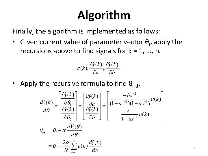
Algorithm Finally, the algorithm is implemented as follows: • Given current value of parameter vector θl, apply the recursions above to find signals for k = 1, …, n. • Apply the recursive formula to find θl+1. 16

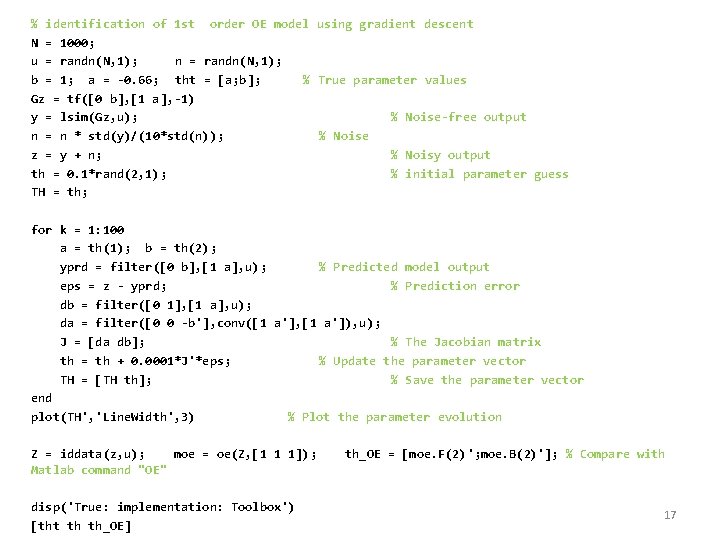
% identification of 1 st order OE model using gradient descent N = 1000; u = randn(N, 1); n = randn(N, 1); b = 1; a = -0. 66; tht = [a; b]; % True parameter values Gz = tf([0 b], [1 a], -1) y = lsim(Gz, u); % Noise-free output n = n * std(y)/(10*std(n)); % Noise z = y + n; % Noisy output th = 0. 1*rand(2, 1); % initial parameter guess TH = th; for k = 1: 100 a = th(1); b = th(2); yprd = filter([0 b], [1 a], u); % Predicted model output eps = z - yprd; % Prediction error db = filter([0 1], [1 a], u); da = filter([0 0 -b'], conv([1 a'], [1 a']), u); J = [da db]; % The Jacobian matrix th = th + 0. 0001*J'*eps; % Update the parameter vector TH = [TH th]; % Save the parameter vector end plot(TH', 'Line. Width', 3) % Plot the parameter evolution Z = iddata(z, u); moe = oe(Z, [1 1 1]); Matlab command "OE" disp('True: implementation: Toolbox') [tht th th_OE] th_OE = [moe. F(2)'; moe. B(2)']; % Compare with 17