Chapter 10 One and TwoSample Tests of Hypotheses

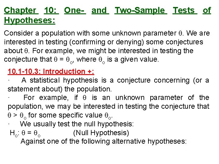
Chapter 10: One- and Two-Sample Tests of Hypotheses: Consider a population with some unknown parameter . We are interested in testing (confirming or denying) some conjectures about . For example, we might be interested in testing the conjecture that = o, where o is a given value. 10. 1 -10. 3: Introduction +: · A statistical hypothesis is a conjecture concerning (or a statement about) the population. · For example, if is an unknown parameter of the population, we may be interested in testing the conjecture that > o for some specific value o. · We usually test the null hypothesis: Ho: = o (Null Hypothesis) Against one of the following alternative hypotheses:

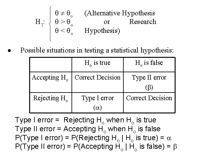
o (Alternative Hypothesis H 1: > o or Research < o Hypothesis) · Possible situations in testing a statistical hypothesis: Ho is true Accepting Ho Correct Decision Rejecting Ho Type I error ( ) Ho is false Type II error ( ) Correct Decision Type I error = Rejecting Ho when Ho is true Type II error = Accepting Ho when Ho is false P(Type I error) = P(Rejecting Ho | Ho is true) = P(Type II error) = P(Accepting Ho | Ho is false) =

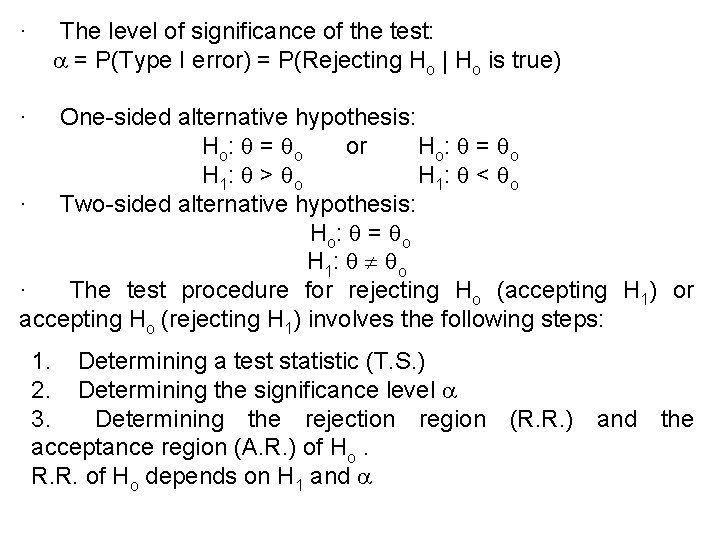
· The level of significance of the test: = P(Type I error) = P(Rejecting Ho | Ho is true) · One-sided alternative hypothesis: Ho: = o or Ho: = o H 1: > o H 1: < o · Two-sided alternative hypothesis: Ho: = o H 1: o · The test procedure for rejecting Ho (accepting H 1) or accepting Ho (rejecting H 1) involves the following steps: 1. Determining a test statistic (T. S. ) 2. Determining the significance level 3. Determining the rejection region (R. R. ) and the acceptance region (A. R. ) of Ho. R. R. of Ho depends on H 1 and

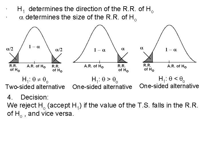
· H 1 determines the direction of the R. R. of Ho · determines the size of the R. R. of Ho H 1: < o H 1: > o Two-sided alternative One-sided alternative 4. Decision: We reject Ho (accept H 1) if the value of the T. S. falls in the R. R. of Ho , and vice versa.

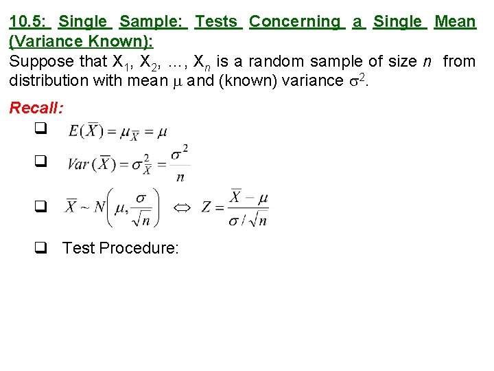
10. 5: Single Sample: Tests Concerning a Single Mean (Variance Known): Suppose that X 1, X 2, …, Xn is a random sample of size n from distribution with mean and (known) variance 2. Recall: q q Test Procedure:

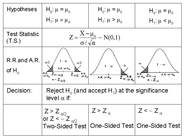
Hypotheses Ho: = o H 1: > o H 1: < o Test Statistic (T. S. ) R. R. and A. R. of Ho Decision: Reject Ho (and accept H 1) at the significance level if: Z > Z Z < Z Z > Z /2 or Z < Z /2 Two-Sided Test One-Sided Test

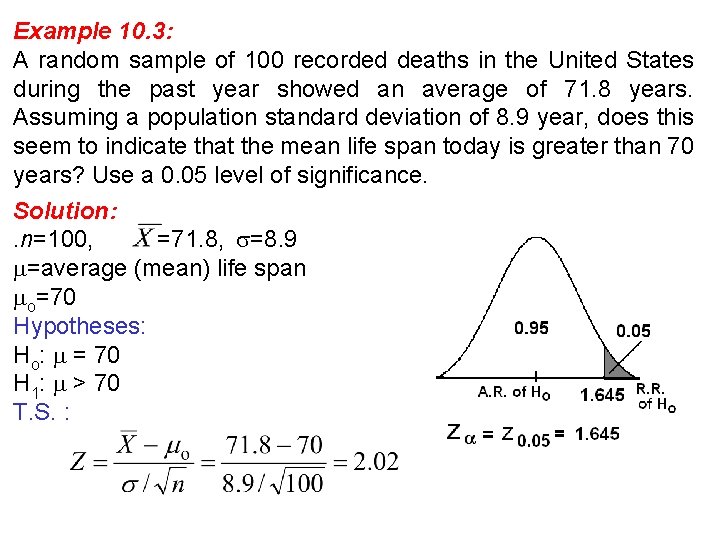
Example 10. 3: A random sample of 100 recorded deaths in the United States during the past year showed an average of 71. 8 years. Assuming a population standard deviation of 8. 9 year, does this seem to indicate that the mean life span today is greater than 70 years? Use a 0. 05 level of significance. Solution: . n=100, =71. 8, =8. 9 =average (mean) life span o=70 Hypotheses: Ho: = 70 H 1: > 70 T. S. :

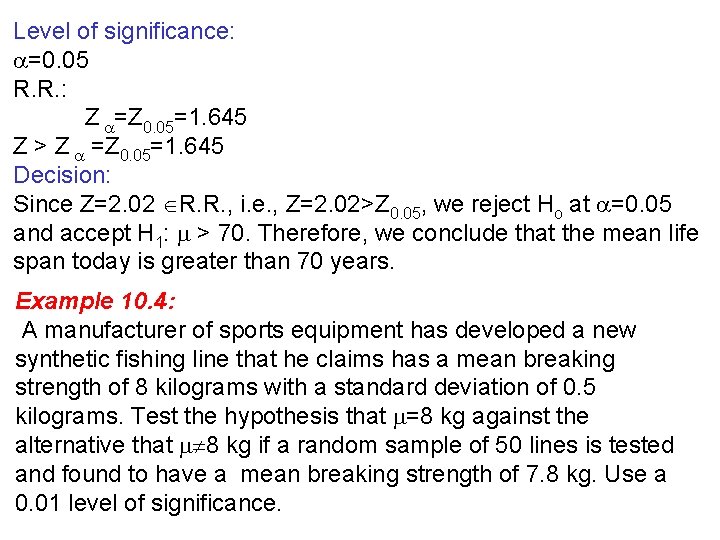
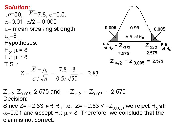
Level of significance: =0. 05 R. R. : Z =Z 0. 05=1. 645 Z > Z =Z 0. 05=1. 645 Decision: Since Z=2. 02 R. R. , i. e. , Z=2. 02>Z 0. 05, we reject Ho at =0. 05 and accept H 1: > 70. Therefore, we conclude that the mean life span today is greater than 70 years. Example 10. 4: A manufacturer of sports equipment has developed a new synthetic fishing line that he claims has a mean breaking strength of 8 kilograms with a standard deviation of 0. 5 kilograms. Test the hypothesis that =8 kg against the alternative that 8 kg if a random sample of 50 lines is tested and found to have a mean breaking strength of 7. 8 kg. Use a 0. 01 level of significance.

Solution: . n=50, =7. 8, =0. 5, =0. 01, /2 = 0. 005 = mean breaking strength o=8 Hypotheses: Ho: = 8 H 1: 8 T. S. : Z /2=Z 0. 005=2. 575 and Z /2= Z 0. 005= 2. 575 Decision: Since Z= 2. 83 R. R. , i. e. , Z= 2. 83 < Z 0. 005, we reject Ho at =0. 01 and accept H 1: 8. Therefore, we conclude that the claim is not correct.

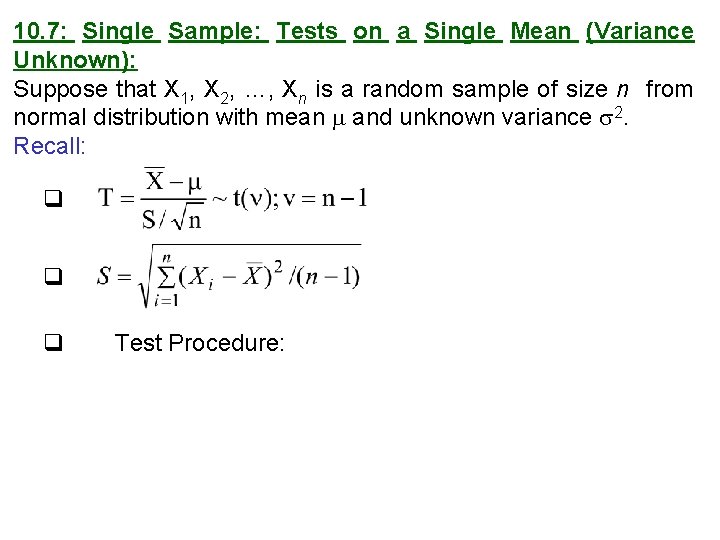
10. 7: Single Sample: Tests on a Single Mean (Variance Unknown): Suppose that X 1, X 2, …, Xn is a random sample of size n from normal distribution with mean and unknown variance 2. Recall: q q q Test Procedure:

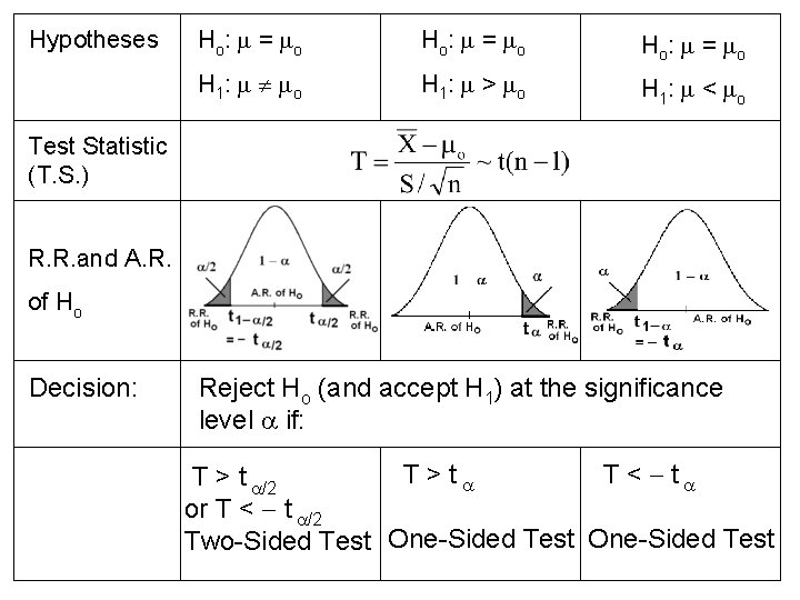
Hypotheses Ho: = o H 1: > o H 1: < o Test Statistic (T. S. ) R. R. and A. R. of Ho Decision: Reject Ho (and accept H 1) at the significance level if: T > t T < t T > t /2 or T < t /2 Two-Sided Test One-Sided Test

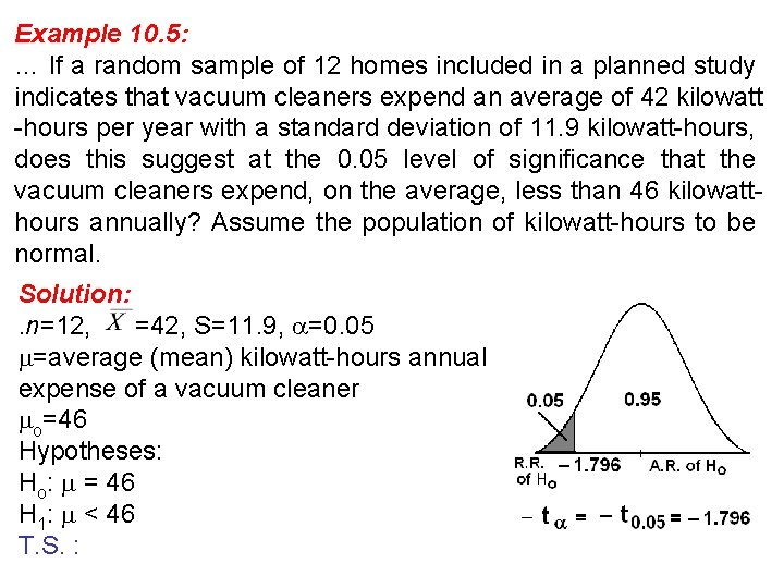
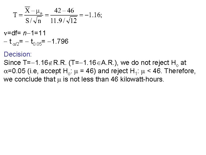
Example 10. 5: … If a random sample of 12 homes included in a planned study indicates that vacuum cleaners expend an average of 42 kilowatt -hours per year with a standard deviation of 11. 9 kilowatt-hours, does this suggest at the 0. 05 level of significance that the vacuum cleaners expend, on the average, less than 46 kilowatthours annually? Assume the population of kilowatt-hours to be normal. Solution: . n=12, =42, S=11. 9, =0. 05 =average (mean) kilowatt-hours annual expense of a vacuum cleaner o=46 Hypotheses: Ho: = 46 H 1: < 46 T. S. :

=df= n 1=11 t /2= t 0. 05= 1. 796 Decision: Since T= 1. 16 R. R. (T= 1. 16 A. R. ), we do not reject Ho at =0. 05 (i. e, accept Ho: = 46) and reject H 1: < 46. Therefore, we conclude that is not less than 46 kilowatt-hours.

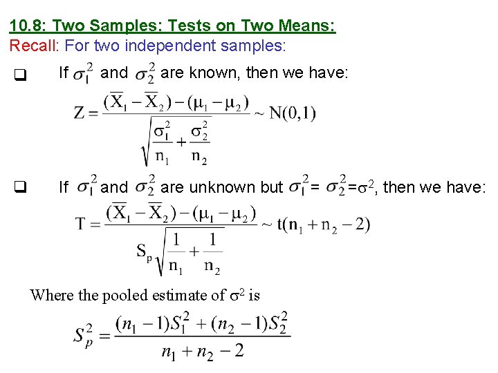
10. 8: Two Samples: Tests on Two Means: Recall: For two independent samples: q If and are known, then we have: q If and are unknown but = = 2, then we have: Where the pooled estimate of 2 is

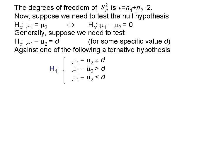
The degrees of freedom of is =n 1+n 2 2. Now, suppose we need to test the null hypothesis Ho: 1 = 2 Ho: 1 2 = 0 Generally, suppose we need to test Ho: 1 2 = d (for some specific value d) Against one of the following alternative hypothesis 1 2 d H 1: 1 2 > d 1 2 < d

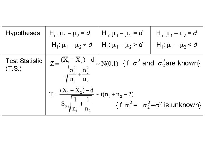
Hypotheses Ho: 1 2 = d H 1: 1 2 d Test Statistic (T. S. ) Ho: 1 2 = d H 1: 1 2 > d H 1: 1 2 < d {if and are known} {if = = 2 is unknown}

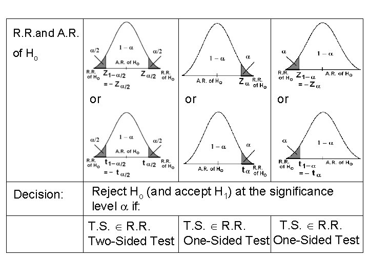
R. R. and A. R. of Ho or Decision: or or Reject Ho (and accept H 1) at the significance level if: T. S. R. R. Two-Sided Test One-Sided Test

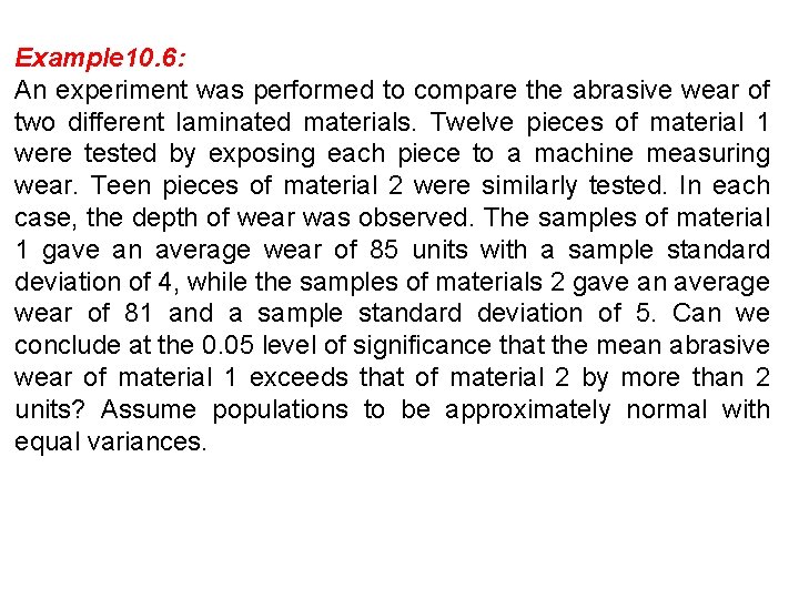
Example 10. 6: An experiment was performed to compare the abrasive wear of two different laminated materials. Twelve pieces of material 1 were tested by exposing each piece to a machine measuring wear. Teen pieces of material 2 were similarly tested. In each case, the depth of wear was observed. The samples of material 1 gave an average wear of 85 units with a sample standard deviation of 4, while the samples of materials 2 gave an average wear of 81 and a sample standard deviation of 5. Can we conclude at the 0. 05 level of significance that the mean abrasive wear of material 1 exceeds that of material 2 by more than 2 units? Assume populations to be approximately normal with equal variances.

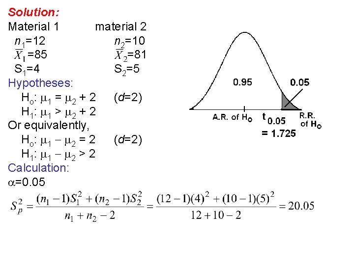
Solution: Material 1 material 2 n 1=12 n 2=10 =85 =81 S 1=4 S 2=5 Hypotheses: Ho: 1 = 2 + 2 (d=2) H 1: 1 > 2 + 2 Or equivalently, Ho: 1 2 = 2 (d=2) H 1: 1 2 > 2 Calculation: =0. 05

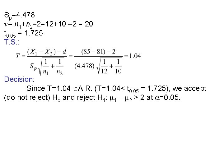
Sp=4. 478 = n 1+n 2 2=12+10 2 = 20 t 0. 05 = 1. 725 T. S. : Decision: Since T=1. 04 A. R. (T=1. 04< t 0. 05 = 1. 725), we accept (do not reject) Ho and reject H 1: 1 2 > 2 at =0. 05.

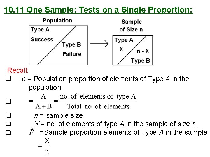
10. 11 One Sample: Tests on a Single Proportion: Recall: q . p = Population proportion of elements of Type A in the population q q n = sample size X = no. of elements of type A in the sample of size n. =Sample proportion elements of Type A in the sample

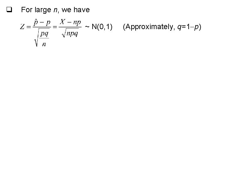
q For large n, we have ~ N(0, 1) (Approximately, q=1 p)

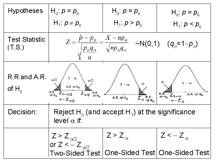
Hypotheses Ho: p = po H 1: p po Test Statistic (T. S. ) Ho: p = po H 1: p > po H 1: p < po ~N(0, 1) (qo=1 po) R. R. and A. R. of Ho Decision: Reject Ho (and accept H 1) at the significance level if: Z > Z Z < Z Z > Z /2 or Z < Z /2 Two-Sided Test One-Sided Test