CHAPTER 10 Market Power Monopoly and Monopsony Copyright

CHAPTER 10 Market Power: Monopoly and Monopsony Copyright © 2013 Pearson Education, Inc. • Microeconomics • Pindyck/Rubinfeld, 8 e. 1 of 52

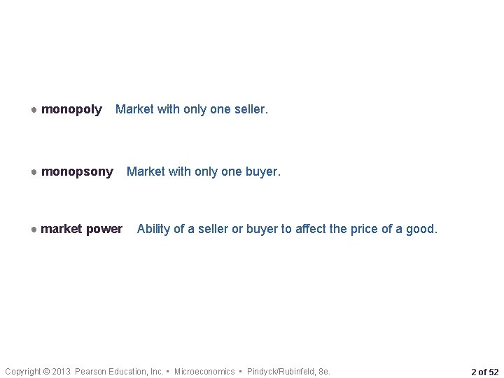
● monopoly Market with only one seller. ● monopsony ● market power Market with only one buyer. Ability of a seller or buyer to affect the price of a good. Copyright © 2013 Pearson Education, Inc. • Microeconomics • Pindyck/Rubinfeld, 8 e. 2 of 52

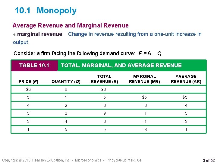
10. 1 Monopoly Average Revenue and Marginal Revenue ● marginal revenue Change in revenue resulting from a one-unit increase in output. Consider a firm facing the following demand curve: P = 6 Q TABLE 10. 1 TOTAL, MARGINAL, AND AVERAGE REVENUE PRICE (P) QUANTITY (Q) TOTAL REVENUE (R) MARGINAL REVENUE (MR) AVERAGE REVENUE (AR) $6 0 $0 — — 5 1 5 $5 $5 4 2 8 3 4 3 3 9 1 3 2 4 8 1 2 1 5 5 3 1 Copyright © 2013 Pearson Education, Inc. • Microeconomics • Pindyck/Rubinfeld, 8 e. 3 of 52

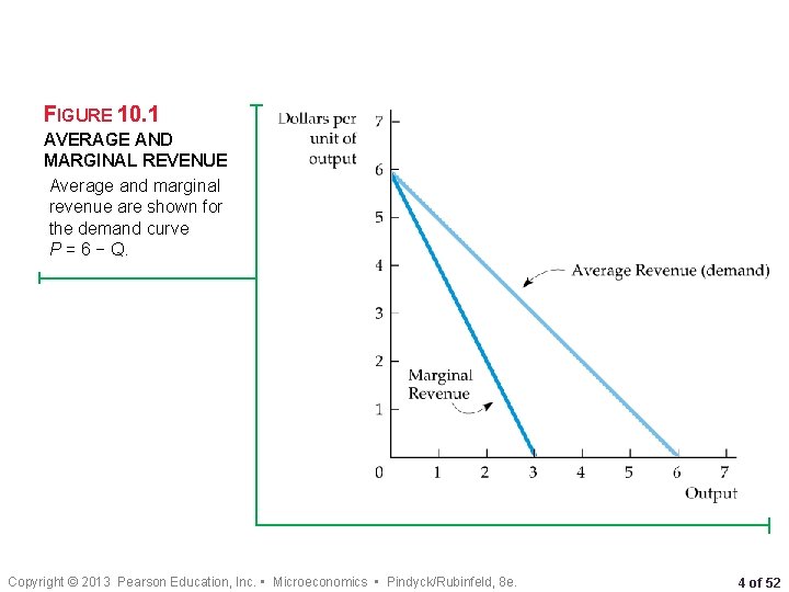
FIGURE 10. 1 AVERAGE AND MARGINAL REVENUE Average and marginal revenue are shown for the demand curve P = 6 − Q. Copyright © 2013 Pearson Education, Inc. • Microeconomics • Pindyck/Rubinfeld, 8 e. 4 of 52

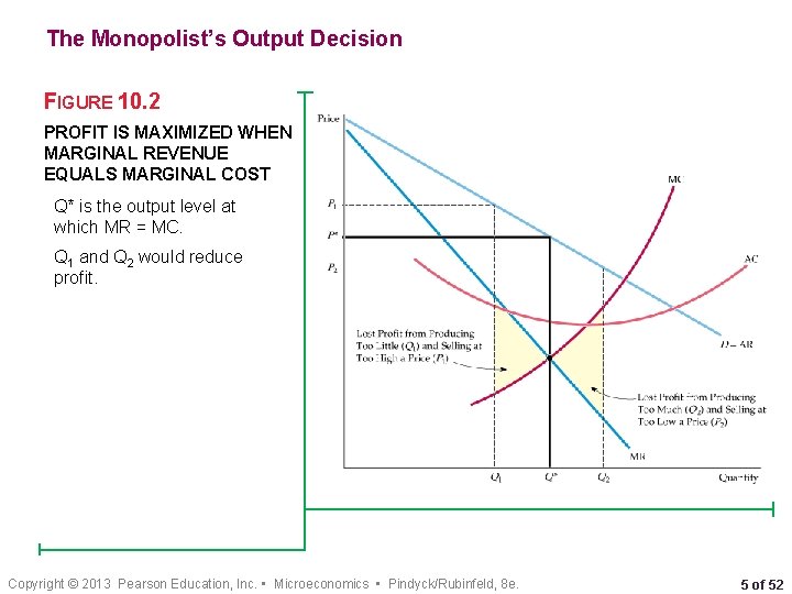
The Monopolist’s Output Decision FIGURE 10. 2 PROFIT IS MAXIMIZED WHEN MARGINAL REVENUE EQUALS MARGINAL COST Q* is the output level at which MR = MC. Q 1 and Q 2 would reduce profit. Copyright © 2013 Pearson Education, Inc. • Microeconomics • Pindyck/Rubinfeld, 8 e. 5 of 52

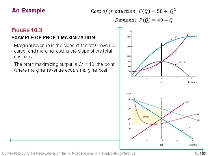
An Example • • FIGURE 10. 3 EXAMPLE OF PROFIT MAXIMIZATION Marginal revenue is the slope of the total revenue curve, and marginal cost is the slope of the total cost curve. The profit-maximizing output is Q* = 10, the point where marginal revenue equals marginal cost. Copyright © 2013 Pearson Education, Inc. • Microeconomics • Pindyck/Rubinfeld, 8 e. 6 of 52

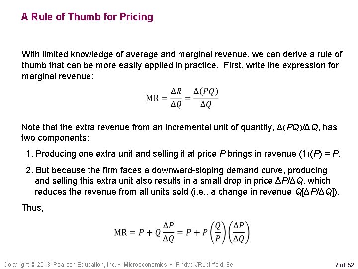
A Rule of Thumb for Pricing With limited knowledge of average and marginal revenue, we can derive a rule of thumb that can be more easily applied in practice. First, write the expression for marginal revenue: • Note that the extra revenue from an incremental unit of quantity, Δ(PQ)/ΔQ, has two components: 1. Producing one extra unit and selling it at price P brings in revenue (1)(P) = P. 2. But because the firm faces a downward-sloping demand curve, producing and selling this extra unit also results in a small drop in price ΔP/ΔQ, which reduces the revenue from all units sold (i. e. , a change in revenue Q[ΔP/ΔQ]). Thus, • Copyright © 2013 Pearson Education, Inc. • Microeconomics • Pindyck/Rubinfeld, 8 e. 7 of 52

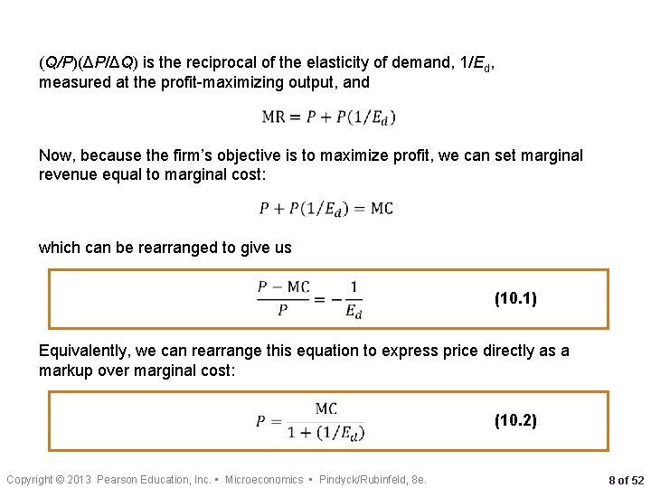
(Q/P)(ΔP/ΔQ) is the reciprocal of the elasticity of demand, 1/Ed, measured at the profit-maximizing output, and • Now, because the firm’s objective is to maximize profit, we can set marginal revenue equal to marginal cost: • which can be rearranged to give us • (10. 1) Equivalently, we can rearrange this equation to express price directly as a markup over marginal cost: • Copyright © 2013 Pearson Education, Inc. • Microeconomics • Pindyck/Rubinfeld, 8 e. (10. 2) 8 of 52

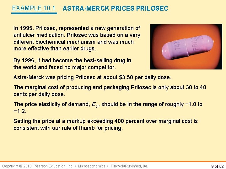
EXAMPLE 10. 1 ASTRA-MERCK PRICES PRILOSEC In 1995, Prilosec, represented a new generation of antiulcer medication. Prilosec was based on a very different biochemical mechanism and was much more effective than earlier drugs. By 1996, it had become the best-selling drug in the world and faced no major competitor. Astra-Merck was pricing Prilosec at about $3. 50 per daily dose. The marginal cost of producing and packaging Prilosec is only about 30 to 40 cents per daily dose. The price elasticity of demand, ED, should be in the range of roughly − 1. 0 to − 1. 2. Setting the price at a markup exceeding 400 percent over marginal cost is consistent with our rule of thumb for pricing. Copyright © 2013 Pearson Education, Inc. • Microeconomics • Pindyck/Rubinfeld, 8 e. 9 of 52

Shifts in Demand A monopolistic market has no supply curve. In other words, there is no one-toone relationship between price and the quantity produced. The reason is that the monopolist’s output decision depends not only on marginal cost but also on the shape of the demand curve. Shifts in demand usually cause changes in both price and quantity. A competitive industry supplies a specific quantity at every price. No such relationship exists for a monopolist, which, depending on how demand shifts, might supply several different quantities at the same price, or the same quantity at different prices. Copyright © 2013 Pearson Education, Inc. • Microeconomics • Pindyck/Rubinfeld, 8 e. 10 of 52

Classwork The perfectly competitive market for carpet has been monopolized (through a series of clever and perhaps illegal buyouts) by the Warm. Toes Carpet Company. Demand for their carpet has been estimated as: P = 40 – 0. 25 Q Where P is price ($/yard) and Q is rate of sales (hundreds of yards per month). Warm. Toes has a total cost curve that is expressed as: TC = 5 Q+. 025 Q 2 • Determine the profit maximizing output rate and price for Warm. Toes. • Determine the rate of profit (or loss) earned by Warm. Toes. • Calculate the welfare changes that result from this monopolization of the market for KP-7. Copyright © 2013 Pearson Education, Inc. • Microeconomics • Pindyck/Rubinfeld, 8 e. 11 of 52

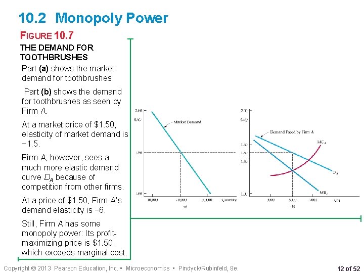
10. 2 Monopoly Power FIGURE 10. 7 THE DEMAND FOR TOOTHBRUSHES Part (a) shows the market demand for toothbrushes. Part (b) shows the demand for toothbrushes as seen by Firm A. At a market price of $1. 50, elasticity of market demand is − 1. 5. Firm A, however, sees a much more elastic demand curve DA because of competition from other firms. At a price of $1. 50, Firm A’s demand elasticity is − 6. Still, Firm A has some monopoly power: Its profitmaximizing price is $1. 50, which exceeds marginal cost. Copyright © 2013 Pearson Education, Inc. • Microeconomics • Pindyck/Rubinfeld, 8 e. 12 of 52

EXAMPLE 10. 2 ELASTICITIES OF DEMAND FOR SOFT DRINKS Soft drinks provide a good example of the difference between a market elasticity of demand a firm’s elasticity of demand. In addition, soft drinks are important because their consumption has been linked to childhood obesity; there could be health benefits from taxing them. A recent review of several statistical studies found that the market elasticity of demand for soft drinks is between − 0. 8 and − 1. 0. 6 That means that if all soft drink producers increased the prices of all of their brands by 1 percent, the quantity of soft drinks demanded would fall by 0. 8 to 1. 0 percent. The demand for any individual soft drink, however, will be much more elastic, because consumers can readily substitute one drink for another. Although elasticities will differ across different brands, studies have shown that the elasticity of demand for, say, Coca Cola is around − 5. 7 In other words, if the price of Coke were increased by 1 percent but the prices of all other soft drinks remained unchanged, the quantity of Coke demanded would fall by about 5 percent. Copyright © 2013 Pearson Education, Inc. • Microeconomics • Pindyck/Rubinfeld, 8 e. 13 of 52

Production, Price, and Monopoly Power In figure 10. 7, although Firm A is not a pure monopolist, it does have monopoly power—it can profitably charge a price greater than marginal cost. Of course, its monopoly power is less than it would be if it had driven away the competition and monopolized the market, but it might still be substantial. This raises two questions. 1. How can we measure monopoly power in order to compare one firm with another? (So far we have been talking about monopoly power only in qualitative terms. ) 2. What are the sources of monopoly power, and why do some firms have more monopoly power than others? Copyright © 2013 Pearson Education, Inc. • Microeconomics • Pindyck/Rubinfeld, 8 e. 14 of 52

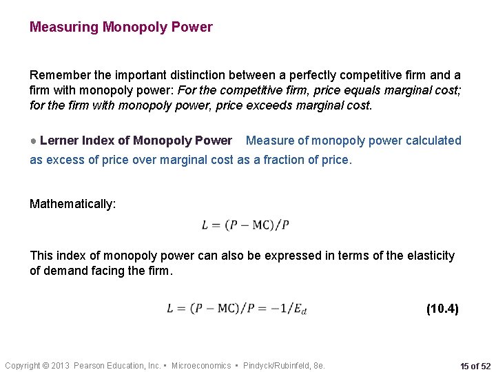
Measuring Monopoly Power Remember the important distinction between a perfectly competitive firm and a firm with monopoly power: For the competitive firm, price equals marginal cost; for the firm with monopoly power, price exceeds marginal cost. ● Lerner Index of Monopoly Power Measure of monopoly power calculated as excess of price over marginal cost as a fraction of price. Mathematically: • This index of monopoly power can also be expressed in terms of the elasticity of demand facing the firm. • Copyright © 2013 Pearson Education, Inc. • Microeconomics • Pindyck/Rubinfeld, 8 e. (10. 4) 15 of 52

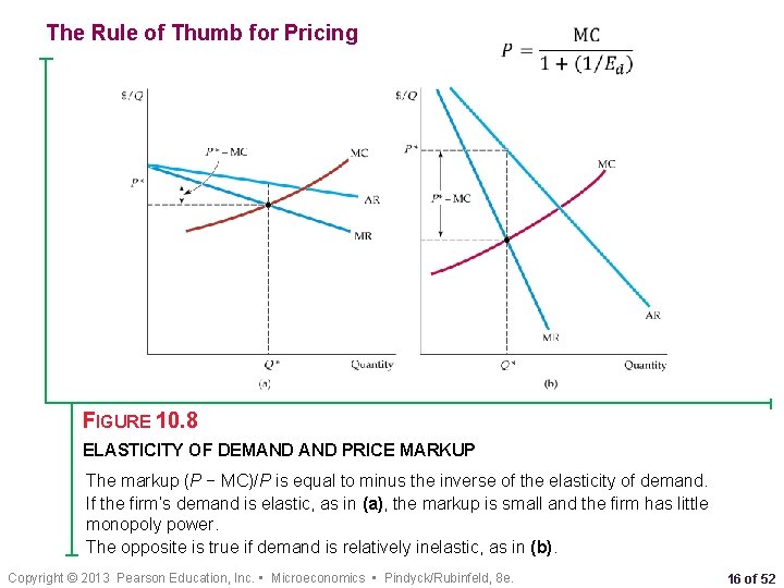
The Rule of Thumb for Pricing • FIGURE 10. 8 ELASTICITY OF DEMAND PRICE MARKUP The markup (P − MC)/P is equal to minus the inverse of the elasticity of demand. If the firm’s demand is elastic, as in (a), the markup is small and the firm has little monopoly power. The opposite is true if demand is relatively inelastic, as in (b). Copyright © 2013 Pearson Education, Inc. • Microeconomics • Pindyck/Rubinfeld, 8 e. 16 of 52

EXAMPLE 10. 3 MARKUP PRICING: SUPERMARKETS TO DESIGNER JEANS Although the elasticity of market demand for food is small (about − 1), no single supermarket can raise its prices very much without losing customers to other stores. The elasticity of demand for any one supermarket is often as large as − 10. We find P = MC/(1 − 0. 1) = MC/(0. 9) = (1. 11)MC. The manager of a typical supermarket should set prices about 11 percent above marginal cost. Small convenience stores typically charge higher prices because its customers are generally less price sensitive. Because the elasticity of demand for a convenience store is about − 5, the markup equation implies that its prices should be about 25 percent above marginal cost. With designer jeans, demand elasticities in the range of − 2 to − 3 are typical. This means that price should be 50 to 100 percent higher than marginal cost. Copyright © 2013 Pearson Education, Inc. • Microeconomics • Pindyck/Rubinfeld, 8 e. 17 of 52

10. 3 Sources of Monopoly Power As equation (10. 4) shows, the less elastic its demand curve, the more monopoly power a firm has. The ultimate determinant of monopoly power is therefore the firm’s elasticity of demand. Three factors determine a firm’s elasticity of demand. 1. The elasticity of market demand. Because the firm’s own demand will be at least as elastic as market demand, the elasticity of market demand limits the potential for monopoly power. 2. The number of firms in the market. If there are many firms, it is unlikely that any one firm will be able to affect price significantly. 3. The interaction among firms. Even if only two or three firms are in the market, each firm will be unable to profitably raise price very much if the rivalry among them is aggressive, with each firm trying to capture as much of the market as it can. Copyright © 2013 Pearson Education, Inc. • Microeconomics • Pindyck/Rubinfeld, 8 e. 18 of 52

The Elasticity of Market Demand If there is only one firm—a pure monopolist—its demand curve is the market demand curve. In this case, the firm’s degree of monopoly power depends completely on the elasticity of market demand. When several firms compete with one another, the elasticity of market demand sets a lower limit on the magnitude of the elasticity of demand for each firm. A particular firm’s elasticity depends on how the firms compete with one another, and the elasticity of market demand limits the potential monopoly power of individual producers. Copyright © 2013 Pearson Education, Inc. • Microeconomics • Pindyck/Rubinfeld, 8 e. 19 of 52

The Number of Firms Other things being equal, the monopoly power of each firm will fall as the number of firms increases. When only a few firms account for most of the sales in a market, we say that the market is highly concentrated. ● barrier to entry Condition that impedes entry by new competitors. Sometimes there are natural barriers to entry: • Patents, copyrights, and licenses • Economies of scale may make it too costly for more than a few firms to supply the entire market. In some cases, economies of scale may be so large that it is most efficient for a single firm—a natural monopoly—to supply the entire market. Copyright © 2013 Pearson Education, Inc. • Microeconomics • Pindyck/Rubinfeld, 8 e. 20 of 52

The Interaction Among Firms might compete aggressively, undercutting one another’s prices to capture more market share, or they might not compete much. They might even collude (in violation of the antitrust laws), agreeing to limit output and raise prices. Other things being equal, monopoly power is smaller when firms compete aggressively and is larger when they cooperate. Because raising prices in concert rather than individually is more likely to be profitable, collusion can generate substantial monopoly power. Furthermore, real or potential monopoly power in the short run can make an industry more competitive in the long run: Large short-run profits can induce new firms to enter an industry, thereby reducing monopoly power over the longer term. Copyright © 2013 Pearson Education, Inc. • Microeconomics • Pindyck/Rubinfeld, 8 e. 21 of 52

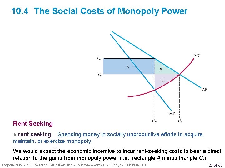
10. 4 The Social Costs of Monopoly Power Rent Seeking ● rent seeking Spending money in socially unproductive efforts to acquire, maintain, or exercise monopoly. We would expect the economic incentive to incur rent-seeking costs to bear a direct relation to the gains from monopoly power (i. e. , rectangle A minus triangle C. ) Copyright © 2013 Pearson Education, Inc. • Microeconomics • Pindyck/Rubinfeld, 8 e. 22 of 52

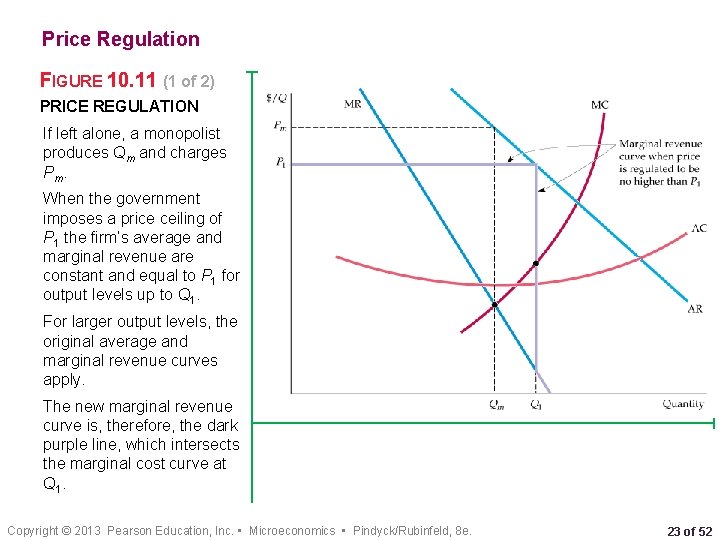
Price Regulation FIGURE 10. 11 (1 of 2) PRICE REGULATION If left alone, a monopolist produces Qm and charges Pm. When the government imposes a price ceiling of P 1 the firm’s average and marginal revenue are constant and equal to P 1 for output levels up to Q 1. For larger output levels, the original average and marginal revenue curves apply. The new marginal revenue curve is, therefore, the dark purple line, which intersects the marginal cost curve at Q 1. Copyright © 2013 Pearson Education, Inc. • Microeconomics • Pindyck/Rubinfeld, 8 e. 23 of 52

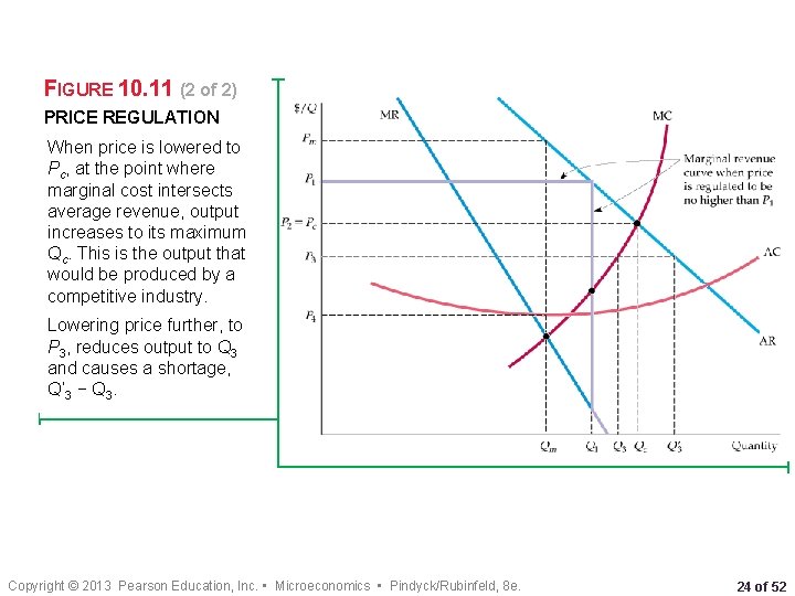
FIGURE 10. 11 (2 of 2) PRICE REGULATION When price is lowered to Pc, at the point where marginal cost intersects average revenue, output increases to its maximum Qc. This is the output that would be produced by a competitive industry. Lowering price further, to P 3, reduces output to Q 3 and causes a shortage, Q’ 3 − Q 3. Copyright © 2013 Pearson Education, Inc. • Microeconomics • Pindyck/Rubinfeld, 8 e. 24 of 52

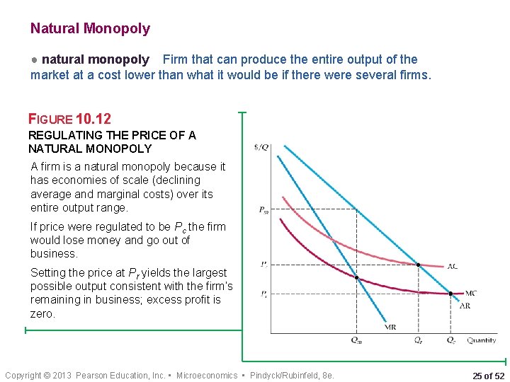
Natural Monopoly ● natural monopoly Firm that can produce the entire output of the market at a cost lower than what it would be if there were several firms. FIGURE 10. 12 REGULATING THE PRICE OF A NATURAL MONOPOLY A firm is a natural monopoly because it has economies of scale (declining average and marginal costs) over its entire output range. If price were regulated to be Pc the firm would lose money and go out of business. Setting the price at Pr yields the largest possible output consistent with the firm’s remaining in business; excess profit is zero. Copyright © 2013 Pearson Education, Inc. • Microeconomics • Pindyck/Rubinfeld, 8 e. 25 of 52

10. 5 Monopsony ● oligopsony Market with only a few buyers. ● monopsony power ● marginal value a good. Buyer’s ability to affect the price of a good. Additional benefit derived from purchasing one more unit of ● marginal expenditure ● average expenditure Additional cost of buying one more unit of a good. Price paid per unit of a good. Copyright © 2013 Pearson Education, Inc. • Microeconomics • Pindyck/Rubinfeld, 8 e. 26 of 52

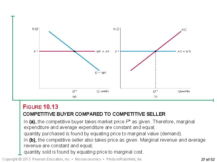
FIGURE 10. 13 COMPETITIVE BUYER COMPARED TO COMPETITIVE SELLER In (a), the competitive buyer takes market price P* as given. Therefore, marginal expenditure and average expenditure are constant and equal; quantity purchased is found by equating price to marginal value (demand). In (b), the competitive seller also takes price as given. Marginal revenue and average revenue are constant and equal; quantity sold is found by equating price to marginal cost. Copyright © 2013 Pearson Education, Inc. • Microeconomics • Pindyck/Rubinfeld, 8 e. 27 of 52

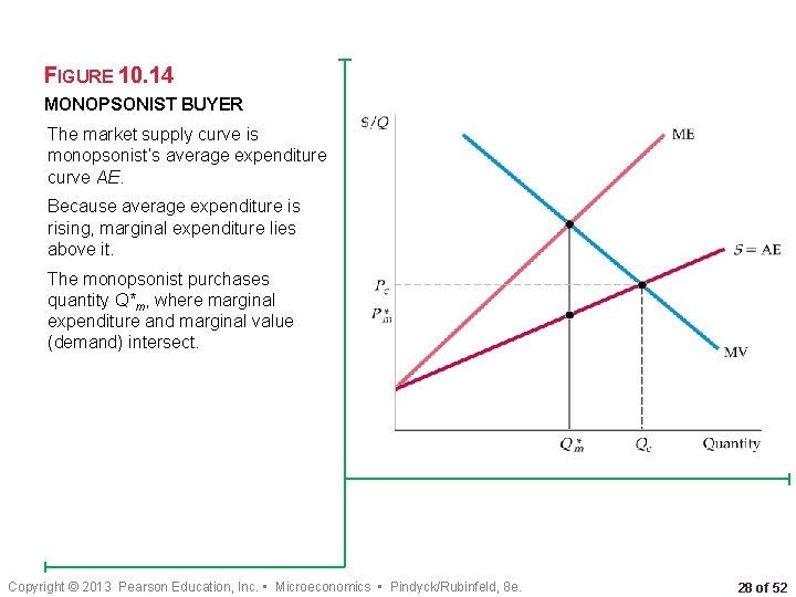
FIGURE 10. 14 MONOPSONIST BUYER The market supply curve is monopsonist’s average expenditure curve AE. Because average expenditure is rising, marginal expenditure lies above it. The monopsonist purchases quantity Q*m, where marginal expenditure and marginal value (demand) intersect. Copyright © 2013 Pearson Education, Inc. • Microeconomics • Pindyck/Rubinfeld, 8 e. 28 of 52

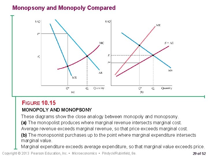
Monopsony and Monopoly Compared FIGURE 10. 15 MONOPOLY AND MONOPSONY These diagrams show the close analogy between monopoly and monopsony. (a) The monopolist produces where marginal revenue intersects marginal cost. Average revenue exceeds marginal revenue, so that price exceeds marginal cost. (b) The monopsonist purchases up to the point where marginal expenditure intersects marginal value. Marginal expenditure exceeds average expenditure, so that marginal value exceeds price. Copyright © 2013 Pearson Education, Inc. • Microeconomics • Pindyck/Rubinfeld, 8 e. 29 of 52