CHAPTER 10 Market Power Monopoly and Monopsony CHAPTER

CHAPTER 10 Market Power: Monopoly and Monopsony CHAPTER OUTLINE 10. 1 Monopoly 10. 2 Monopoly Power 10. 3 Sources of Monopoly Power 10. 4 The Social Costs of Monopoly Power Prepared by: Fernando Quijano, Illustrator Copyright © 2013 Pearson Education, Inc. • Microeconomics • Pindyck/Rubinfeld, 8 e. 1 of 52

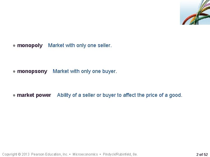
● monopoly Market with only one seller. ● monopsony ● market power Market with only one buyer. Ability of a seller or buyer to affect the price of a good. Copyright © 2013 Pearson Education, Inc. • Microeconomics • Pindyck/Rubinfeld, 8 e. 2 of 52

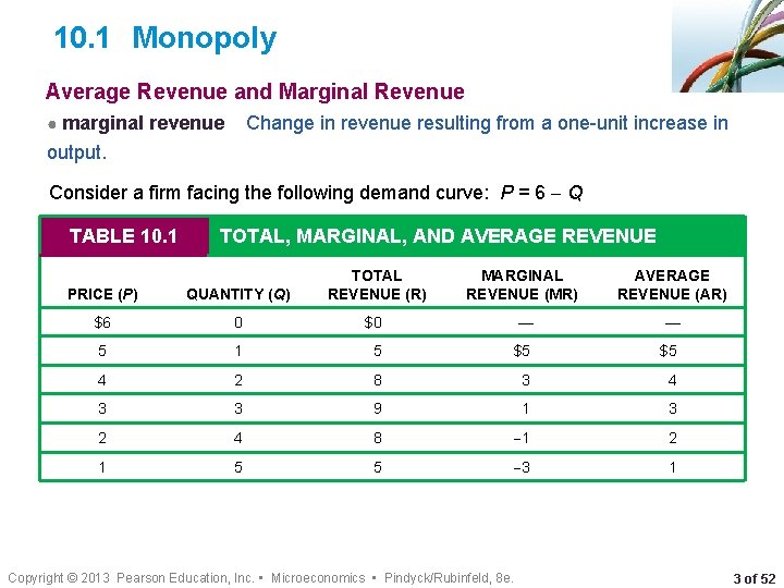
10. 1 Monopoly Average Revenue and Marginal Revenue ● marginal revenue Change in revenue resulting from a one-unit increase in output. Consider a firm facing the following demand curve: P = 6 Q TABLE 10. 1 TOTAL, MARGINAL, AND AVERAGE REVENUE PRICE (P) QUANTITY (Q) TOTAL REVENUE (R) MARGINAL REVENUE (MR) AVERAGE REVENUE (AR) $6 0 $0 — — 5 1 5 $5 $5 4 2 8 3 4 3 3 9 1 3 2 4 8 1 2 1 5 5 3 1 Copyright © 2013 Pearson Education, Inc. • Microeconomics • Pindyck/Rubinfeld, 8 e. 3 of 52

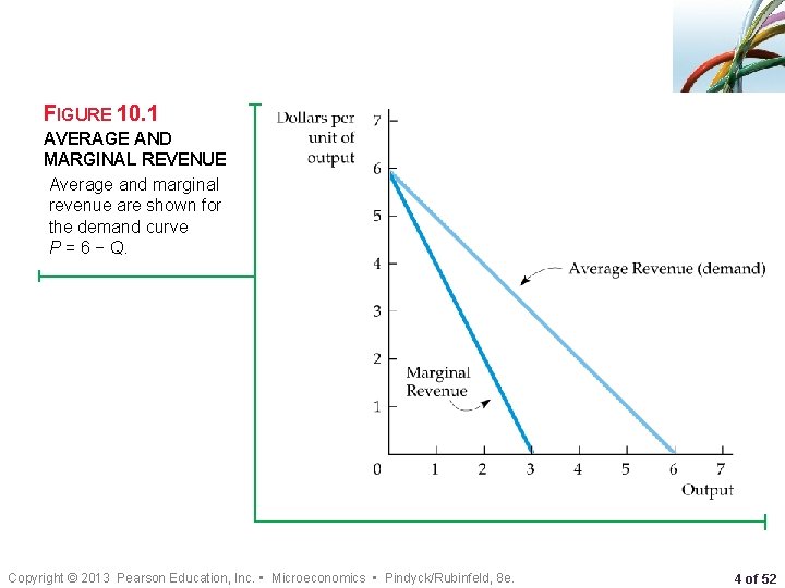
FIGURE 10. 1 AVERAGE AND MARGINAL REVENUE Average and marginal revenue are shown for the demand curve P = 6 − Q. Copyright © 2013 Pearson Education, Inc. • Microeconomics • Pindyck/Rubinfeld, 8 e. 4 of 52

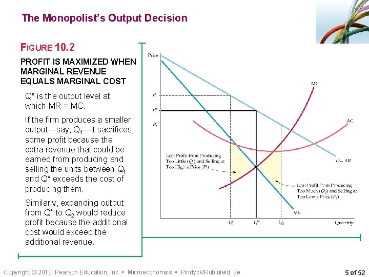
The Monopolist’s Output Decision FIGURE 10. 2 PROFIT IS MAXIMIZED WHEN MARGINAL REVENUE EQUALS MARGINAL COST Q* is the output level at which MR = MC. If the firm produces a smaller output—say, Q 1—it sacrifices some profit because the extra revenue that could be earned from producing and selling the units between Q 1 and Q* exceeds the cost of producing them. Similarly, expanding output from Q* to Q 2 would reduce profit because the additional cost would exceed the additional revenue. Copyright © 2013 Pearson Education, Inc. • Microeconomics • Pindyck/Rubinfeld, 8 e. 5 of 52

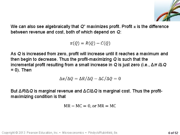
We can also see algebraically that Q* maximizes profit. Profit π is the difference between revenue and cost, both of which depend on Q: • As Q is increased from zero, profit will increase until it reaches a maximum and then begin to decrease. Thus the profit-maximizing Q is such that the incremental profit resulting from a small increase in Q is just zero (i. e. , Δπ /ΔQ = 0). Then • But ΔR/ΔQ is marginal revenue and ΔC/ΔQ is marginal cost. Thus the profitmaximizing condition is that • Copyright © 2013 Pearson Education, Inc. • Microeconomics • Pindyck/Rubinfeld, 8 e. 6 of 52

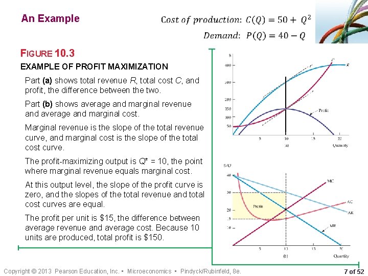
An Example • • FIGURE 10. 3 EXAMPLE OF PROFIT MAXIMIZATION Part (a) shows total revenue R, total cost C, and profit, the difference between the two. Part (b) shows average and marginal revenue and average and marginal cost. Marginal revenue is the slope of the total revenue curve, and marginal cost is the slope of the total cost curve. The profit-maximizing output is Q* = 10, the point where marginal revenue equals marginal cost. At this output level, the slope of the profit curve is zero, and the slopes of the total revenue and total cost curves are equal. The profit per unit is $15, the difference between average revenue and average cost. Because 10 units are produced, total profit is $150. Copyright © 2013 Pearson Education, Inc. • Microeconomics • Pindyck/Rubinfeld, 8 e. 7 of 52

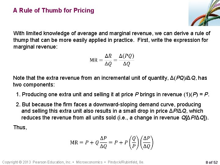
A Rule of Thumb for Pricing With limited knowledge of average and marginal revenue, we can derive a rule of thump that can be more easily applied in practice. First, write the expression for marginal revenue: • Note that the extra revenue from an incremental unit of quantity, Δ(PQ)/ΔQ, has two components: 1. Producing one extra unit and selling it at price P brings in revenue (1)(P) = P. 2. But because the firm faces a downward-sloping demand curve, producing and selling this extra unit also results in a small drop in price ΔP/ΔQ, which reduces the revenue from all units sold (i. e. , a change in revenue Q[ΔP/ΔQ]). Thus, • Copyright © 2013 Pearson Education, Inc. • Microeconomics • Pindyck/Rubinfeld, 8 e. 8 of 52

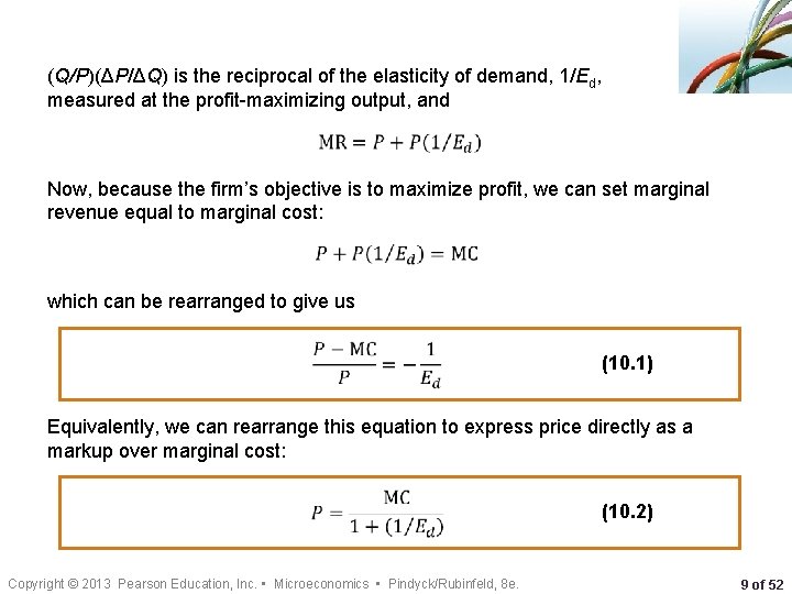
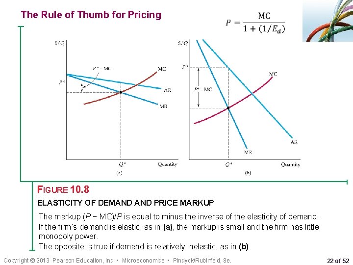
(Q/P)(ΔP/ΔQ) is the reciprocal of the elasticity of demand, 1/Ed, measured at the profit-maximizing output, and • Now, because the firm’s objective is to maximize profit, we can set marginal revenue equal to marginal cost: • which can be rearranged to give us • (10. 1) Equivalently, we can rearrange this equation to express price directly as a markup over marginal cost: • Copyright © 2013 Pearson Education, Inc. • Microeconomics • Pindyck/Rubinfeld, 8 e. (10. 2) 9 of 52

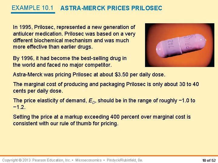
EXAMPLE 10. 1 ASTRA-MERCK PRICES PRILOSEC In 1995, Prilosec, represented a new generation of antiulcer medication. Prilosec was based on a very different biochemical mechanism and was much more effective than earlier drugs. By 1996, it had become the best-selling drug in the world and faced no major competitor. Astra-Merck was pricing Prilosec at about $3. 50 per daily dose. The marginal cost of producing and packaging Prilosec is only about 30 to 40 cents per daily dose. The price elasticity of demand, ED, should be in the range of roughly − 1. 0 to − 1. 2. Setting the price at a markup exceeding 400 percent over marginal cost is consistent with our rule of thumb for pricing. Copyright © 2013 Pearson Education, Inc. • Microeconomics • Pindyck/Rubinfeld, 8 e. 10 of 52

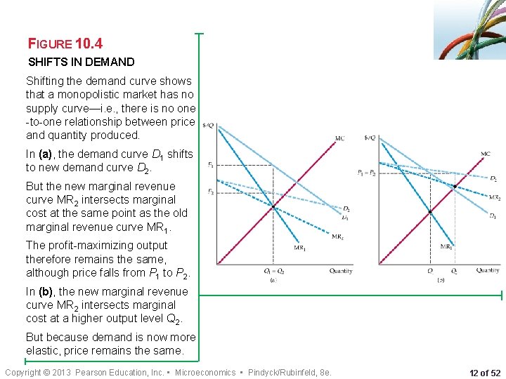
Shifts in Demand A monopolistic market has no supply curve. In other words, there is no one-toone relationship between price and the quantity produced. The reason is that the monopolist’s output decision depends not only on marginal cost but also on the shape of the demand curve. As a result, shifts in demand do not trace out the series of prices and quantities that correspond to a competitive supply curve. Instead, shifts in demand can lead to changes in price with no change in output, changes in output with no change in price, or changes in both price and output. Shifts in demand usually cause changes in both price and quantity. A competitive industry supplies a specific quantity at every price. No such relationship exists for a monopolist, which, depending on how demand shifts, might supply several different quantities at the same price, or the same quantity at different prices. Copyright © 2013 Pearson Education, Inc. • Microeconomics • Pindyck/Rubinfeld, 8 e. 11 of 52

FIGURE 10. 4 SHIFTS IN DEMAND Shifting the demand curve shows that a monopolistic market has no supply curve—i. e. , there is no one -to-one relationship between price and quantity produced. In (a), the demand curve D 1 shifts to new demand curve D 2. But the new marginal revenue curve MR 2 intersects marginal cost at the same point as the old marginal revenue curve MR 1. The profit-maximizing output therefore remains the same, although price falls from P 1 to P 2. In (b), the new marginal revenue curve MR 2 intersects marginal cost at a higher output level Q 2. But because demand is now more elastic, price remains the same. Copyright © 2013 Pearson Education, Inc. • Microeconomics • Pindyck/Rubinfeld, 8 e. 12 of 52

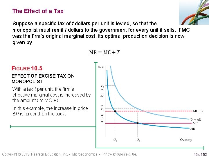
The Effect of a Tax Suppose a specific tax of t dollars per unit is levied, so that the monopolist must remit t dollars to the government for every unit it sells. If MC was the firm’s original marginal cost, its optimal production decision is now given by • FIGURE 10. 5 EFFECT OF EXCISE TAX ON MONOPOLIST With a tax t per unit, the firm’s effective marginal cost is increased by the amount t to MC + t. In this example, the increase in price ΔP is larger than the tax t. Copyright © 2013 Pearson Education, Inc. • Microeconomics • Pindyck/Rubinfeld, 8 e. 13 of 52

The Multiplant Firm Suppose a firm has two plants. What should its total output be, and how much of that output should each plant produce? We can find the answer intuitively in two steps. ● Step 1. Whatever the total output, it should be divided between the two plants so that marginal cost is the same in each plant. Otherwise, the firm could reduce its costs and increase its profit by reallocating production. ● Step 2. We know that total output must be such that marginal revenue equals marginal cost. Otherwise, the firm could increase its profit by raising or lowering total output. Copyright © 2013 Pearson Education, Inc. • Microeconomics • Pindyck/Rubinfeld, 8 e. 14 of 52

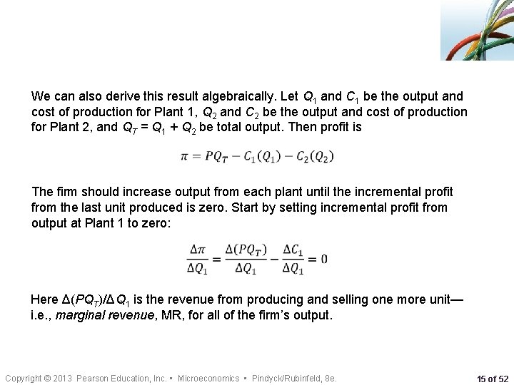
We can also derive this result algebraically. Let Q 1 and C 1 be the output and cost of production for Plant 1, Q 2 and C 2 be the output and cost of production for Plant 2, and QT = Q 1 + Q 2 be total output. Then profit is • The firm should increase output from each plant until the incremental profit from the last unit produced is zero. Start by setting incremental profit from output at Plant 1 to zero: • Here Δ(PQT)/ΔQ 1 is the revenue from producing and selling one more unit— i. e. , marginal revenue, MR, for all of the firm’s output. Copyright © 2013 Pearson Education, Inc. • Microeconomics • Pindyck/Rubinfeld, 8 e. 15 of 52

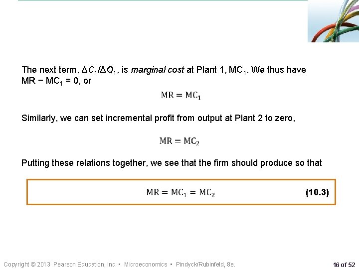
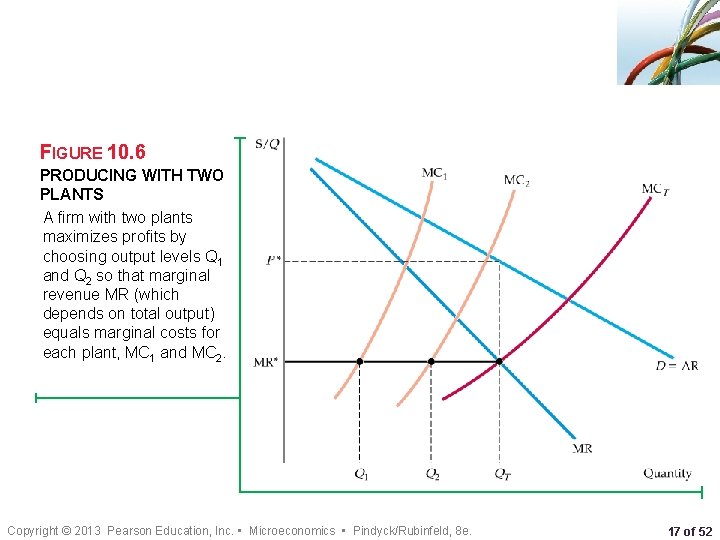
The next term, ΔC 1/ΔQ 1, is marginal cost at Plant 1, MC 1. We thus have MR − MC 1 = 0, or • Similarly, we can set incremental profit from output at Plant 2 to zero, • Putting these relations together, we see that the firm should produce so that • Copyright © 2013 Pearson Education, Inc. • Microeconomics • Pindyck/Rubinfeld, 8 e. (10. 3) 16 of 52

FIGURE 10. 6 PRODUCING WITH TWO PLANTS A firm with two plants maximizes profits by choosing output levels Q 1 and Q 2 so that marginal revenue MR (which depends on total output) equals marginal costs for each plant, MC 1 and MC 2. Copyright © 2013 Pearson Education, Inc. • Microeconomics • Pindyck/Rubinfeld, 8 e. 17 of 52

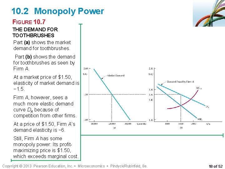
10. 2 Monopoly Power FIGURE 10. 7 THE DEMAND FOR TOOTHBRUSHES Part (a) shows the market demand for toothbrushes. Part (b) shows the demand for toothbrushes as seen by Firm A. At a market price of $1. 50, elasticity of market demand is − 1. 5. Firm A, however, sees a much more elastic demand curve DA because of competition from other firms. At a price of $1. 50, Firm A’s demand elasticity is − 6. Still, Firm A has some monopoly power: Its profitmaximizing price is $1. 50, which exceeds marginal cost. Copyright © 2013 Pearson Education, Inc. • Microeconomics • Pindyck/Rubinfeld, 8 e. 18 of 52

EXAMPLE 10. 2 ELASTICITIES OF DEMAND FOR SOFT DRINKS Soft drinks provide a good example of the difference between a market elasticity of demand a firm’s elasticity of demand. In addition, soft drinks are important because their consumption has been linked to childhood obesity; there could be health benefits from taxing them. A recent review of several statistical studies found that the market elasticity of demand for soft drinks is between − 0. 8 and − 1. 0. 6 That means that if all soft drink producers increased the prices of all of their brands by 1 percent, the quantity of soft drinks demanded would fall by 0. 8 to 1. 0 percent. The demand for any individual soft drink, however, will be much more elastic, because consumers can readily substitute one drink for another. Although elasticities will differ across different brands, studies have shown that the elasticity of demand for, say, Coca Cola is around − 5. 7 In other words, if the price of Coke were increased by 1 percent but the prices of all other soft drinks remained unchanged, the quantity of Coke demanded would fall by about 5 percent. Students—and business people—sometimes confuse the market elasticity of demand with the firm (or brand) elasticity of demand. Make sure you understand the difference. Copyright © 2013 Pearson Education, Inc. • Microeconomics • Pindyck/Rubinfeld, 8 e. 19 of 52

Production, Price, and Monopoly Power In figure 10. 7, although Firm A is not a pure monopolist, it does have monopoly power—it can profitably charge a price greater than marginal cost. Of course, its monopoly power is less than it would be if it had driven away the competition and monopolized the market, but it might still be substantial. This raises two questions. 1. How can we measure monopoly power in order to compare one firm with another? (So far we have been talking about monopoly power only in qualitative terms. ) 2. What are the sources of monopoly power, and why do some firms have more monopoly power than others? We address both these questions below, although a more complete answer to the second question will be provided in Chapters 12 and 13. Copyright © 2013 Pearson Education, Inc. • Microeconomics • Pindyck/Rubinfeld, 8 e. 20 of 52

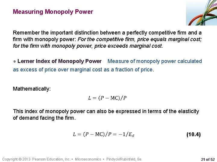
Measuring Monopoly Power Remember the important distinction between a perfectly competitive firm and a firm with monopoly power: For the competitive firm, price equals marginal cost; for the firm with monopoly power, price exceeds marginal cost. ● Lerner Index of Monopoly Power Measure of monopoly power calculated as excess of price over marginal cost as a fraction of price. Mathematically: • This index of monopoly power can also be expressed in terms of the elasticity of demand facing the firm. • Copyright © 2013 Pearson Education, Inc. • Microeconomics • Pindyck/Rubinfeld, 8 e. (10. 4) 21 of 52

The Rule of Thumb for Pricing • FIGURE 10. 8 ELASTICITY OF DEMAND PRICE MARKUP The markup (P − MC)/P is equal to minus the inverse of the elasticity of demand. If the firm’s demand is elastic, as in (a), the markup is small and the firm has little monopoly power. The opposite is true if demand is relatively inelastic, as in (b). Copyright © 2013 Pearson Education, Inc. • Microeconomics • Pindyck/Rubinfeld, 8 e. 22 of 52

EXAMPLE 10. 3 MARKUP PRICING: SUPERMARKETS TO DESIGNER JEANS Although the elasticity of market demand for food is small (about − 1), no single supermarket can raise its prices very much without losing customers to other stores. The elasticity of demand for any one supermarket is often as large as − 10. We find P = MC/(1 − 0. 1) = MC/(0. 9) = (1. 11)MC. The manager of a typical supermarket should set prices about 11 percent above marginal cost. Small convenience stores typically charge higher prices because its customers are generally less price sensitive. Because the elasticity of demand for a convenience store is about − 5, the markup equation implies that its prices should be about 25 percent above marginal cost. With designer jeans, demand elasticities in the range of − 2 to − 3 are typical. This means that price should be 50 to 100 percent higher than marginal cost. Copyright © 2013 Pearson Education, Inc. • Microeconomics • Pindyck/Rubinfeld, 8 e. 23 of 52

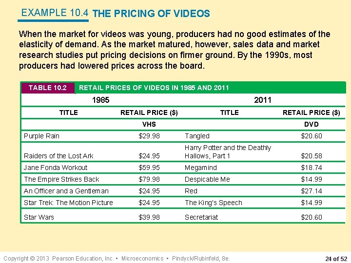
EXAMPLE 10. 4 THE PRICING OF VIDEOS When the market for videos was young, producers had no good estimates of the elasticity of demand. As the market matured, however, sales data and market research studies put pricing decisions on firmer ground. By the 1990 s, most producers had lowered prices across the board. TABLE 10. 2 RETAIL PRICES OF VIDEOS IN 1985 AND 2011 1985 TITLE 2011 RETAIL PRICE ($) TITLE VHS Purple Rain RETAIL PRICE ($) DVD $29. 98 Tangled $20. 60 Raiders of the Lost Ark $24. 95 Harry Potter and the Deathly Hallows, Part 1 $20. 58 Jane Fonda Workout $59. 95 Megamind $18. 74 The Empire Strikes Back $79. 98 Despicable Me $14. 99 An Officer and a Gentleman $24. 95 Red $27. 14 Star Trek: The Motion Picture $24. 95 The King’s Speech $14. 99 Star Wars $39. 98 Secretariat $20. 60 Copyright © 2013 Pearson Education, Inc. • Microeconomics • Pindyck/Rubinfeld, 8 e. 24 of 52

EXAMPLE 10. 4 THE PRICING OF VIDEOS FIGURE 10. 9 VIDEO SALES Between 1990 and 1998, lower prices induced consumers to buy many more videos. By 2001, sales of DVDs overtook sales of VHS videocassettes. High-definition DVDs were introduced in 2006, and are expected to displace sales of conventional DVDs. All DVDs, however, are now being displaced by streaming video. Copyright © 2013 Pearson Education, Inc. • Microeconomics • Pindyck/Rubinfeld, 8 e. 25 of 52

10. 3 Sources of Monopoly Power As equation (10. 4) shows, the less elastic its demand curve, the more monopoly power a firm has. The ultimate determinant of monopoly power is therefore the firm’s elasticity of demand. Three factors determine a firm’s elasticity of demand. 1. The elasticity of market demand. Because the firm’s own demand will be at least as elastic as market demand, the elasticity of market demand limits the potential for monopoly power. 2. The number of firms in the market. If there are many firms, it is unlikely that any one firm will be able to affect price significantly. 3. The interaction among firms. Even if only two or three firms are in the market, each firm will be unable to profitably raise price very much if the rivalry among them is aggressive, with each firm trying to capture as much of the market as it can. Copyright © 2013 Pearson Education, Inc. • Microeconomics • Pindyck/Rubinfeld, 8 e. 26 of 52

The Elasticity of Market Demand If there is only one firm—a pure monopolist—its demand curve is the market demand curve. In this case, the firm’s degree of monopoly power depends completely on the elasticity of market demand. When several firms compete with one another, the elasticity of market demand sets a lower limit on the magnitude of the elasticity of demand for each firm. A particular firm’s elasticity depends on how the firms compete with one another, and the elasticity of market demand limits the potential monopoly power of individual producers. Because the demand for oil is fairly inelastic (at least in the short run), OPEC could raise oil prices far above marginal production cost during the 1970 s and early 1980 s. Because the demands for such commodities as coffee, cocoa, tin, and copper are much more elastic, attempts by producers to cartelize these markets and raise prices have largely failed. In each case, the elasticity of market demand limits the potential monopoly power of individual producers. Copyright © 2013 Pearson Education, Inc. • Microeconomics • Pindyck/Rubinfeld, 8 e. 27 of 52

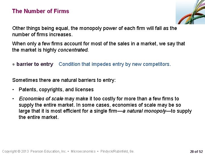
The Number of Firms Other things being equal, the monopoly power of each firm will fall as the number of firms increases. When only a few firms account for most of the sales in a market, we say that the market is highly concentrated. ● barrier to entry Condition that impedes entry by new competitors. Sometimes there are natural barriers to entry: • Patents, copyrights, and licenses • Economies of scale may make it too costly for more than a few firms to supply the entire market. In some cases, economies of scale may be so large that it is most efficient for a single firm—a natural monopoly—to supply the entire market. Copyright © 2013 Pearson Education, Inc. • Microeconomics • Pindyck/Rubinfeld, 8 e. 28 of 52

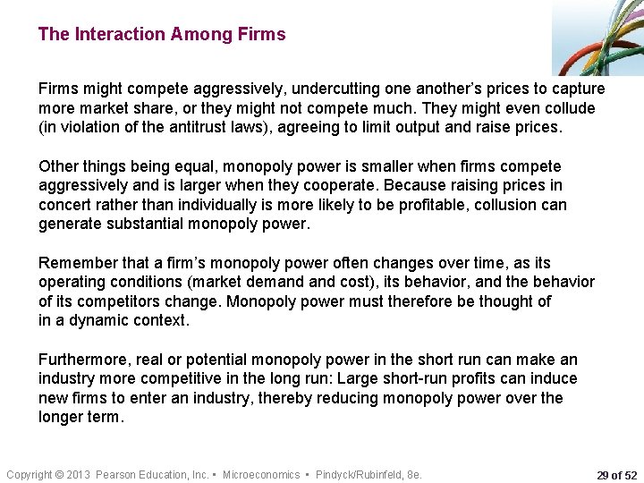
The Interaction Among Firms might compete aggressively, undercutting one another’s prices to capture more market share, or they might not compete much. They might even collude (in violation of the antitrust laws), agreeing to limit output and raise prices. Other things being equal, monopoly power is smaller when firms compete aggressively and is larger when they cooperate. Because raising prices in concert rather than individually is more likely to be profitable, collusion can generate substantial monopoly power. Remember that a firm’s monopoly power often changes over time, as its operating conditions (market demand cost), its behavior, and the behavior of its competitors change. Monopoly power must therefore be thought of in a dynamic context. Furthermore, real or potential monopoly power in the short run can make an industry more competitive in the long run: Large short-run profits can induce new firms to enter an industry, thereby reducing monopoly power over the longer term. Copyright © 2013 Pearson Education, Inc. • Microeconomics • Pindyck/Rubinfeld, 8 e. 29 of 52

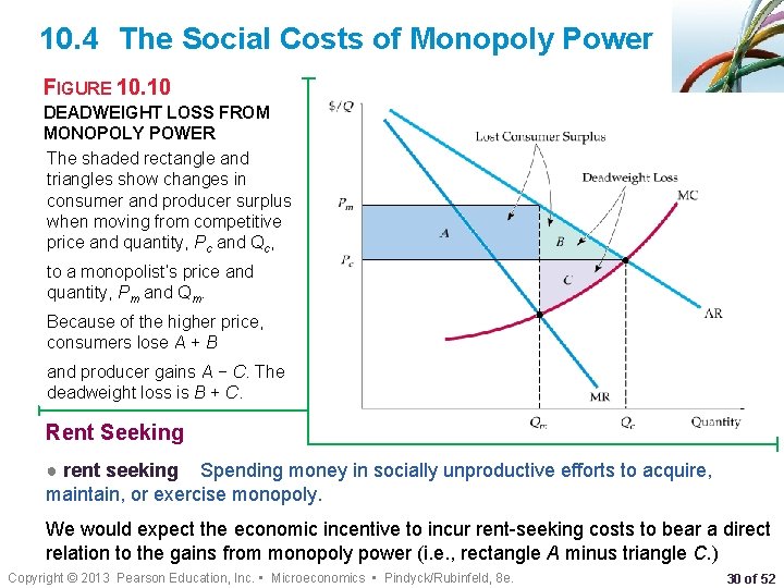
10. 4 The Social Costs of Monopoly Power FIGURE 10. 10 DEADWEIGHT LOSS FROM MONOPOLY POWER The shaded rectangle and triangles show changes in consumer and producer surplus when moving from competitive price and quantity, Pc and Qc, to a monopolist’s price and quantity, Pm and Qm. Because of the higher price, consumers lose A + B and producer gains A − C. The deadweight loss is B + C. Rent Seeking ● rent seeking Spending money in socially unproductive efforts to acquire, maintain, or exercise monopoly. We would expect the economic incentive to incur rent-seeking costs to bear a direct relation to the gains from monopoly power (i. e. , rectangle A minus triangle C. ) Copyright © 2013 Pearson Education, Inc. • Microeconomics • Pindyck/Rubinfeld, 8 e. 30 of 52

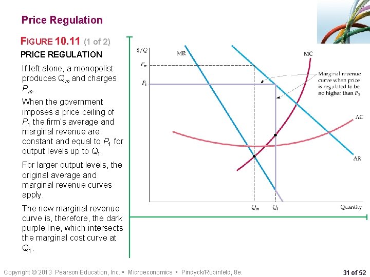
Price Regulation FIGURE 10. 11 (1 of 2) PRICE REGULATION If left alone, a monopolist produces Qm and charges Pm. When the government imposes a price ceiling of P 1 the firm’s average and marginal revenue are constant and equal to P 1 for output levels up to Q 1. For larger output levels, the original average and marginal revenue curves apply. The new marginal revenue curve is, therefore, the dark purple line, which intersects the marginal cost curve at Q 1. Copyright © 2013 Pearson Education, Inc. • Microeconomics • Pindyck/Rubinfeld, 8 e. 31 of 52

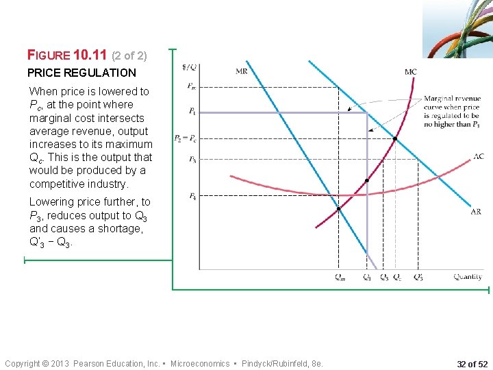
FIGURE 10. 11 (2 of 2) PRICE REGULATION When price is lowered to Pc, at the point where marginal cost intersects average revenue, output increases to its maximum Qc. This is the output that would be produced by a competitive industry. Lowering price further, to P 3, reduces output to Q 3 and causes a shortage, Q’ 3 − Q 3. Copyright © 2013 Pearson Education, Inc. • Microeconomics • Pindyck/Rubinfeld, 8 e. 32 of 52

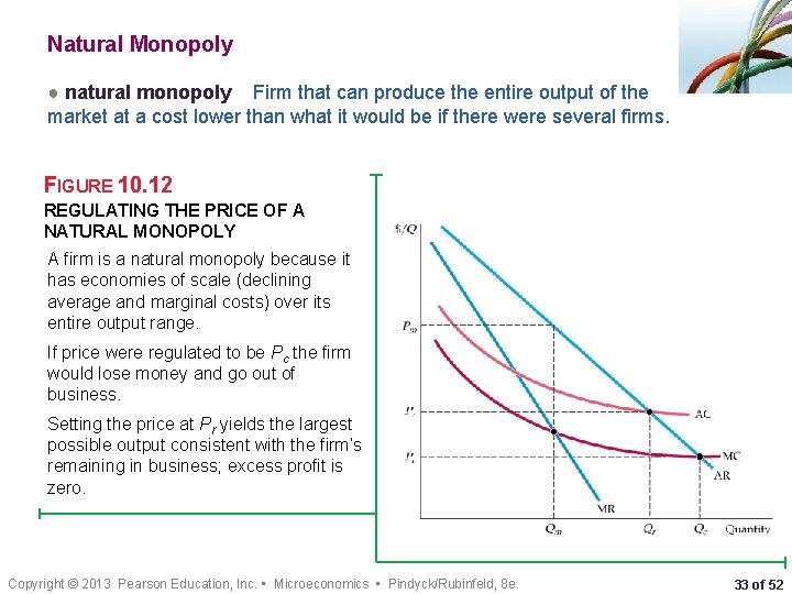
Natural Monopoly ● natural monopoly Firm that can produce the entire output of the market at a cost lower than what it would be if there were several firms. FIGURE 10. 12 REGULATING THE PRICE OF A NATURAL MONOPOLY A firm is a natural monopoly because it has economies of scale (declining average and marginal costs) over its entire output range. If price were regulated to be Pc the firm would lose money and go out of business. Setting the price at Pr yields the largest possible output consistent with the firm’s remaining in business; excess profit is zero. Copyright © 2013 Pearson Education, Inc. • Microeconomics • Pindyck/Rubinfeld, 8 e. 33 of 52

Regulation in Practice The regulation of a monopoly is sometimes based on the rate of return that it earns on its capital. The regulatory agency determines an allowed price, so that this rate of return is in some sense “competitive” or “fair. ” ● rate-of-return regulation Maximum price allowed by a regulatory agency is based on the (expected) rate of return that a firm will earn. Although it is a key element in determining the firm’s rate of return, a firm’s capital stock is difficult to value. While a “fair” rate of return must be based on the firm’s actual cost of capital, that cost depends in turn on the behavior of the regulatory agency. Regulatory lag is a term associated with delays in changing regulated prices. Another approach to regulation is setting price caps based on the firm’s variable costs. A price cap can allow for more flexibility than rate-of-return regulation. Under price cap regulation, for example, a firm would typically be allowed to raise its prices each year (without having to get approval from the regulatory agency) by an amount equal to the actual rate of inflation, minus expected productivity growth. Copyright © 2013 Pearson Education, Inc. • Microeconomics • Pindyck/Rubinfeld, 8 e. 34 of 52