Acceleration Polygon for a CrankSlider Introduction Acceleration Polygon

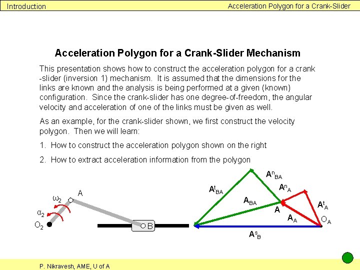
Acceleration Polygon for a Crank-Slider Introduction Acceleration Polygon for a Crank-Slider Mechanism This presentation shows how to construct the acceleration polygon for a crank -slider (inversion 1) mechanism. It is assumed that the dimensions for the links are known and the analysis is being performed at a given (known) configuration. Since the crank-slider has one degree-of-freedom, the angular velocity and acceleration of one of the links must be given as well. As an example, for the crank-slider shown, we first construct the velocity polygon. Then we will learn: 1. How to construct the acceleration polygon shown on the right 2. How to extract acceleration information from the polygon An. BA ω2 An A At. BA A ABA α 2 O 2 P. Nikravesh, AME, U of A B As. B A At. A AA OA

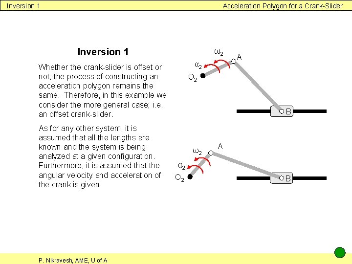
Inversion 1 Acceleration Polygon for a Crank-Slider Inversion 1 ω2 α 2 Whether the crank-slider is offset or not, the process of constructing an acceleration polygon remains the same. Therefore, in this example we consider the more general case; i. e. , an offset crank-slider. As for any other system, it is assumed that all the lengths are known and the system is being analyzed at a given configuration. Furthermore, it is assumed that the angular velocity and acceleration of the crank is given. P. Nikravesh, AME, U of A A O 2 B ω2 A α 2 O 2 B

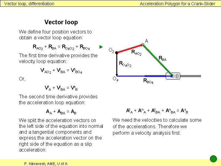
Vector loop, differentiation Acceleration Polygon for a Crank-Slider Vector loop We define four position vectors to obtain a vector loop equation: RAO 2 + RBA = RO 4 O 2 + RBO 4 A ► The first time derivative provides the velocity loop equation: O 2 RBA RO 4 O 2 Vt. AO 2 + Vt. BA = Vs. BO 4 Or, RAO 2 RBO 4 B Vt. A + Vt. BA = Vs. B The second time derivative provides the acceleration loop equation: AA + ABA = AB At. A + An. A + At. BA + An. BA = As. B We split the acceleration vectors on the left side of the equation into normal and a tangential components and express the acceleration vector on the right side of the equation as a slip acceleration: We need the velocities to calculate some of the accelerations. Therefore we perform a velocity analysis first. P. Nikravesh, AME, U of A

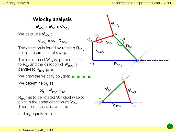
Velocity analysis Acceleration Polygon for a Crank-Slider Velocity analysis Vt. AO 2 + Vt. BA = Vt. AO 2 Vs. BO 4 We calculate Vt. AO 2 : Vt. AO 2 = ω2 ∙ RAO 2 The direction is found by rotating RAO 2 90° in the direction of ω2 ► The direction of Vt. BA is perpendicular to RBA and the direction of Vs. BO 4 is parallel to RBO 4 ► ► A ω2 O 4 A Vt. BA ω3 = Vt. BA / RBA P. Nikravesh, AME, U of A B RBO 4 We determine ω3 as: and ω4 equals zero. RBA RO 4 O 2 We draw the velocity polygon: ► ► RBA has to be rotated 90° clockwise to point in the same direction as Vt. BA. Therefore ω3 is clockwise ► ω3 RAO 2 Vt. AO 2 B Vs. BO 4 OV

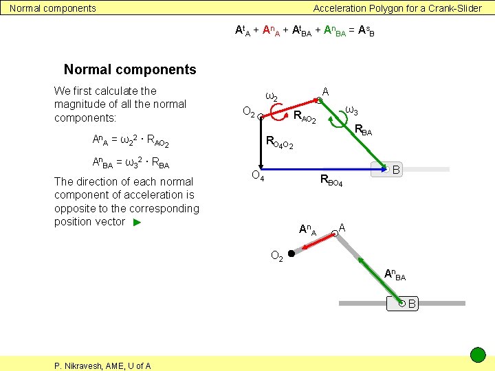
Normal components Acceleration Polygon for a Crank-Slider At. A + An. A + At. BA + An. BA = As. B Normal components We first calculate the magnitude of all the normal components: An A O 2 = ω2 ∙ RAO 2 2 An. BA = ω32 ∙ RBA The direction of each normal component of acceleration is opposite to the corresponding position vector ► A ω2 ω3 RAO 2 RBA RO 4 O 2 O 4 RBO 4 An A B A O 2 An. BA B P. Nikravesh, AME, U of A

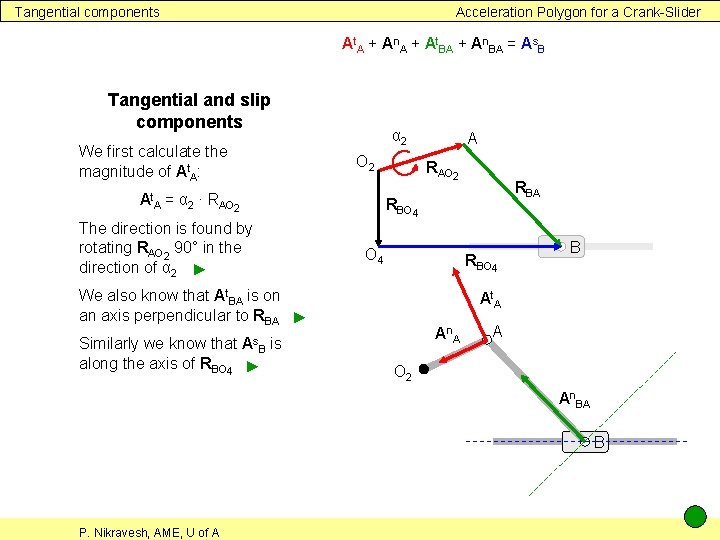
Tangential components Acceleration Polygon for a Crank-Slider At. A + An. A + At. BA + An. BA = As. B Tangential and slip components We first calculate the magnitude of At. A: α 2 O 2 At. A = α 2 ∙ RAO 2 A RAO 2 RBA RBO 4 The direction is found by rotating RAO 2 90° in the direction of α 2 ► O 4 RBO 4 We also know that At. BA is on an axis perpendicular to RBA ► Similarly we know that is along the axis of RBO 4 ► B At. A An A As. B A O 2 An. BA B P. Nikravesh, AME, U of A

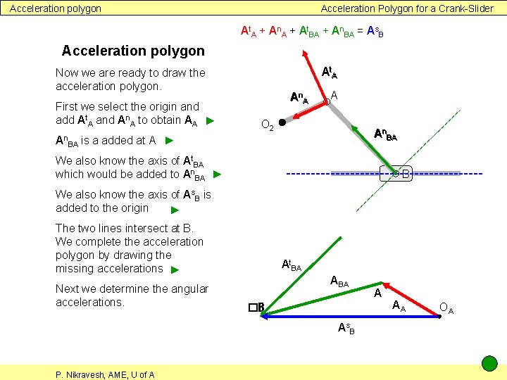
Acceleration polygon Acceleration Polygon for a Crank-Slider At. A + An. A + At. BA + An. BA = As. B Acceleration polygon At. A Now we are ready to draw the acceleration polygon. First we select the origin and add At. A and An. A to obtain AA ► An BA An A A O 2 An. BA is a added at A ► We also know the axis of At. BA which would be added to An. BA ► B We also know the axis of As. B is added to the origin ► The two lines intersect at B. We complete the acceleration polygon by drawing the missing accelerations ► Next we determine the angular accelerations. An. BA An A At. BA ABA �B As. B P. Nikravesh, AME, U of A A At. A AA OA

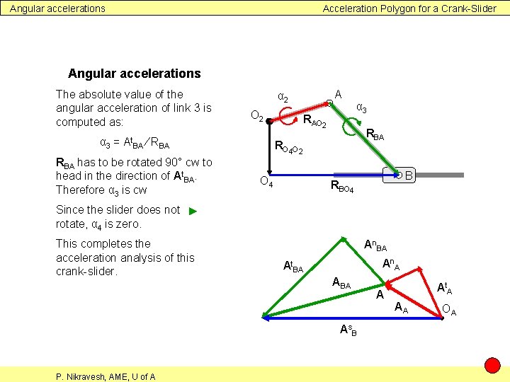
Angular accelerations Acceleration Polygon for a Crank-Slider Angular accelerations The absolute value of the angular acceleration of link 3 is computed as: O 2 α 3 = At. BA ∕ RBA has to be rotated 90° cw to head in the direction of At. BA. Therefore α 3 is cw A α 2 RAO 2 α 3 RBA RO 4 O 2 O 4 B RBO 4 Since the slider does not ► rotate, α 4 is zero. This completes the acceleration analysis of this crank-slider. An. BA An A At. BA As. B P. Nikravesh, AME, U of A A At. A AA OA