5 April 2005 Copulas 101 on Copulas in

5 April 2005 Copulas 101 on Copulas in MS Excel for insurance projects Lucas du Croo de Jongh, Matt Leonard, Arjun Raychaudhuri CONFIDENTIAL LON-TCJ 00111 -034

Confidentiality Our clients’ industries are extremely competitive. The confidentiality of companies’ plans and data is obviously critical. Mercer Oliver Wyman will protect the confidentiality of all such client information. Similarly, management consulting is a competitive business. We view our approaches and insights as proprietary and therefore look to our clients to protect Mercer Oliver Wyman interests in our presentations, methodologies and analytical techniques. Under no circumstances should this material be shared with any third party without the written consent of Mercer Oliver Wyman. Copyright © 2005 Mercer Oliver Wyman LON-TCJ 00111 -034

– Draft – This document provides an practical guide to copulas Addressed questions – What is a copula? – When should I use a copula? o In what ways are copulas alternatives to (and improvements on) existing techniques that we (MOW) traditionally use? What are the pros and cons? o Are copulas usually associated with some modelling approaches and not others (e. g. are copulas more commonly used in DFA-type models? ) o How should I approach it in a client setting? – How do I apply a copula? o How should I select a copula? o How do I parameterise a copula (in MS Excel)? o How do I sample a copula (in MS Excel)? – Where can I learn more? o Who are the contact people in the insurance domain? o What articles should I read? Suggestions for improvement to this document are appreciated (e. g. , examples, client material) LON-TCJ 00111 -034 2 Copyright © 2005 Mercer Oliver Wyman n

– Draft – Contents 1. When to use a copula 2. The mathematics of copulas 3. A list of useful copulas 4. Calibrating a copula – Visualization – Parameterization 5. Sampling a copula 6. Further considerations on tail dependencies 7. References Copyright © 2005 Mercer Oliver Wyman LON-TCJ 00111 -034 3

– Draft – Section 1 When to use a copula Copyright © 2005 Mercer Oliver Wyman LON-TCJ 00111 -034 4

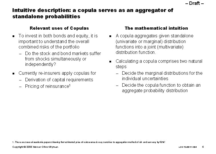
– Draft – Intuitive description: a copula serves as an aggregator of standalone probabilities Relevant uses of Copulas n n To invest in both bonds and equity, it is important to understand the overall combined risks of the portfolio – Do the stock and bond markets suffer from shocks simultaneously or independently? Currently re-insurers apply copulas for – Derivation of capital requirements – Pricing of reinsurance 1 The mathematical intuition n n A copula aggregates given standalone (univariate or marginal) distribution functions into a joint (multivariate) distribution function. Calculating a copula comprises two natural steps – Decide the marginal distributions for the individual uncertainties – Decide the copula function to obtain an aggregate probability distribution 1. There are several academic papers showing that estimated price of reinsurance is very sensitive to aggregation method of risk and can vary by 50%! Copyright © 2005 Mercer Oliver Wyman LON-TCJ 00111 -034 5

– Draft – Both Gaussians and Copulas have their benefits Copyright © 2005 Mercer Oliver Wyman LON-TCJ 00111 -034 6

– Draft – Guidelines: only apply copulas if they have substantial and sustainable advantage over Gaussians – UNDER CONSTRUCTION n n n Benefits of copulas have to be material to the client and have to be among the top improvements in pricing (e. g. for reinsurance) or risk management The organisation has to be able to absorb this added complexity; enough people have to be able to calibrate, operate and interpret the results from the model Implementation need to be accompanied by intuitive sanity checks at several stages E. g. , output of var-covar matrices, diagrams to depict dependencies etc. Upon implementation user should always start with Gaussian copulas and check output before moving on to other copulas It is strongly recommendable to use the T-copula, as it preserves some of the nice features of Gaussians copulas. E. g. , correlation matrices (which can be calibrated using a closed formula) Copyright © 2005 Mercer Oliver Wyman LON-TCJ 00111 -034 7

– Draft – Section 2 The mathematics of copulas Copyright © 2005 Mercer Oliver Wyman LON-TCJ 00111 -034 8

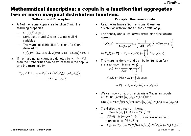
– Draft – Mathematical description: a copula is a function that aggregates two or more marginal distribution functions Mathematical Description n A N-dimensional copula is a function C with the following properties – – – n and C is increasing in all N Example: Gaussian copula n n variables The marginal distribution functions for C are denoted by If the marginal functions are denoted by then the probabilities can be expressed in the copula and the marginals by n n n Assume we have a 2 -dimensional Gaussian distribution with variance 1 and correlation ρ. The density and (cumulative) distribution function are known: The marginal density and distribution function for x are also known (same for y) We can now construct the bivariate Gaussian copula C: Define then C satisfies the three conditions: – – variables as . C is increasing in both is – Copyright © 2005 Mercer Oliver Wyman LON-TCJ 00111 -034 9

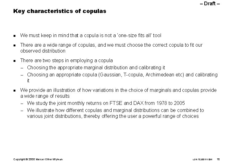
– Draft – Key characteristics of copulas n n We must keep in mind that a copula is not a ‘one-size fits all’ tool There a wide range of copulas, and we must choose the correct copula to fit our observed distribution There are two steps in employing a copula – Choosing the appropriate marginal distribution and calibrating it – Choosing an appropriate copula (Gaussian, T-copula, Archimedean etc) and calibrating it We provide an illustration of how variations in the choice of marginals and copulas provide a wide range of results – We study the joint monthly returns on FTSE and DAX from 1978 to 2005 – We illustrate how different copulas and marginal distributions can be combined to various joint distributions, thereby offering the user a powerful range of choices Copyright © 2005 Mercer Oliver Wyman LON-TCJ 00111 -034 10

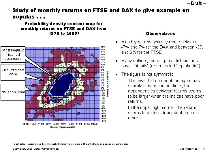
– Draft – Study of monthly returns on FTSE and DAX to give example on copulas. . . Probability density contour map for monthly returns on FTSE and DAX from 1978 to 20051 Observations n Most frequent historical occurrence Occurred only once Never occurred 1 n n Monthly returns typically range between -7% and 7% for the DAX and between -3% and 6% for the FTSE Many outliers; the marginal distributions have “fat tails” (or are called “leptokurtic”) The figure is not symmetric – The lower left corner of the figure has sharply curved contour lines; the dependencies between returns seems to be larger when the indices have poor returns – In the upper right corner, the returns seems to be less dependent on each other Each colour represents a different probability density as if it were a different altitude on a geological contour map Copyright © 2005 Mercer Oliver Wyman LON-TCJ 00111 -034 11

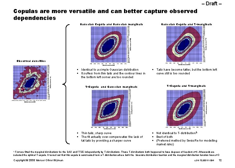
– Draft – Copulas are more versatile and can better capture observed dependencies Gaussian Copula and Gaussian marginals Gaussian Copula and T-marginals Observed densities § Identical to a simple Gaussian distribution § It suffers from thin tails and the contour lines in the bottom left corner are too rounded T-Copula and Gaussian marginals § Thin tails, sharp curve § The fit actually over-compensates the lack of fat tails by providing a sharper curve § Tails have become fatter, but the bottom left curve still is too rounded T-Copula and T-marginals § Not identical to T-distribution 1) § Best of both § (Preferred method by Swiss. Re for modelling market risks) First we fitted the marginal distributions for the DAX and FTSE independently by T-distributions. These T-distributions both happened to have degrees of freedom ν=4. Afterwards we selected the optimal T-copula. It turned out that this copula is constructed from a T-distribution where both the bivariate distribution fucntion and the marginal distribution function have ν=3 1 Copyright © 2005 Mercer Oliver Wyman LON-TCJ 00111 -034 12

– Draft – Section 3 A list of useful copulas Copyright © 2005 Mercer Oliver Wyman LON-TCJ 00111 -034 13

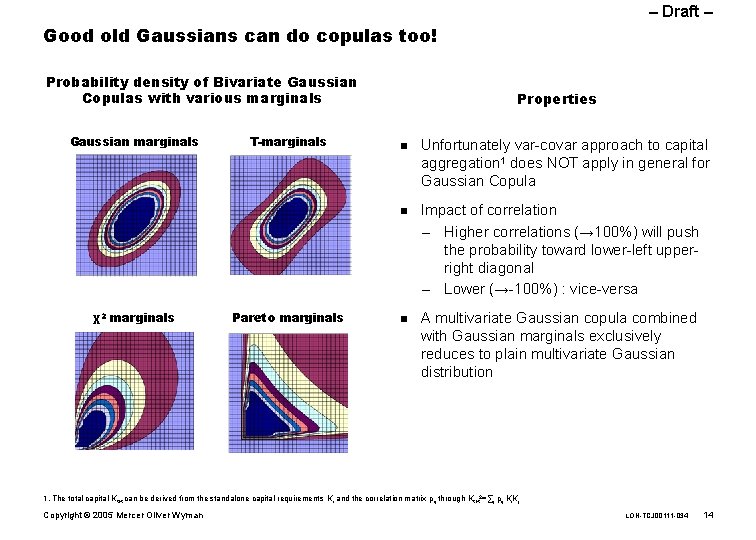
– Draft – Good old Gaussians can do copulas too! Probability density of Bivariate Gaussian Copulas with various marginals Gaussian marginals T-marginals Properties n n χ2 marginals Pareto marginals n Unfortunately var-covar approach to capital aggregation 1 does NOT apply in general for Gaussian Copula Impact of correlation – Higher correlations (→ 100%) will push the probability toward lower-left upperright diagonal – Lower (→-100%) : vice-versa A multivariate Gaussian copula combined with Gaussian marginals exclusively reduces to plain multivariate Gaussian distribution 1. The total capital Ktot can be derived from the standalone capital requirements Ki and the correlation matrix ρij through Ktot 2=∑ij ρij Ki. Kj Copyright © 2005 Mercer Oliver Wyman LON-TCJ 00111 -034 14

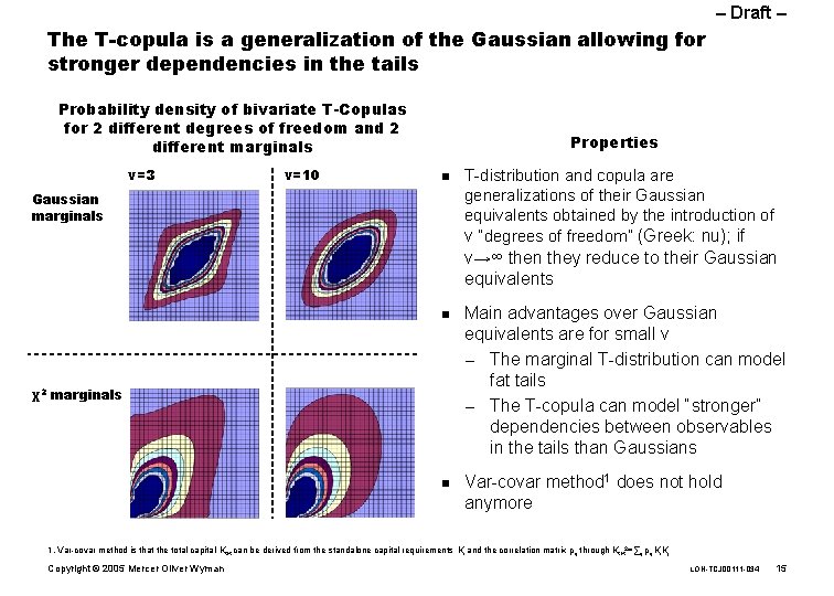
– Draft – The T-copula is a generalization of the Gaussian allowing for stronger dependencies in the tails Probability density of bivariate T-Copulas for 2 different degrees of freedom and 2 different marginals ν=3 ν=10 Properties n Gaussian marginals T-distribution and copula are generalizations of their Gaussian equivalents obtained by the introduction of ν “degrees of freedom” (Greek: nu); if ν→∞ then they reduce to their Gaussian equivalents n χ2 marginals n Main advantages over Gaussian equivalents are for small v – The marginal T-distribution can model fat tails – The T-copula can model “stronger” dependencies between observables in the tails than Gaussians Var-covar method 1 does not hold anymore 1. Var-covar method is that the total capital Ktot can be derived from the standalone capital requirements Ki and the correlation matrix ρij through Ktot 2=∑ij ρij Ki. Kj Copyright © 2005 Mercer Oliver Wyman LON-TCJ 00111 -034 15

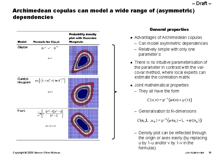
– Draft – Archimedean copulas can model a wide range of (asymmetric) dependencies General properties n n n Advantages of Archimedean copulas – Can model asymmetric dependencies – Relatively simple with only one parameter α There is no intuitive parameterisation of the parameter in contrast with the varcovar method, where local experts can estimate the correlation matrix Joint mathematical properties – They all have the form – Generalisation to N-dimensions – Density plot can be reflected through the origin or axes easily (by replacing u by 1 -u and/or v by 1 -v in the formulas) Copyright © 2005 Mercer Oliver Wyman LON-TCJ 00111 -034 16

– Draft – Section 4 Calibrating a copula Copyright © 2005 Mercer Oliver Wyman LON-TCJ 00111 -034 17

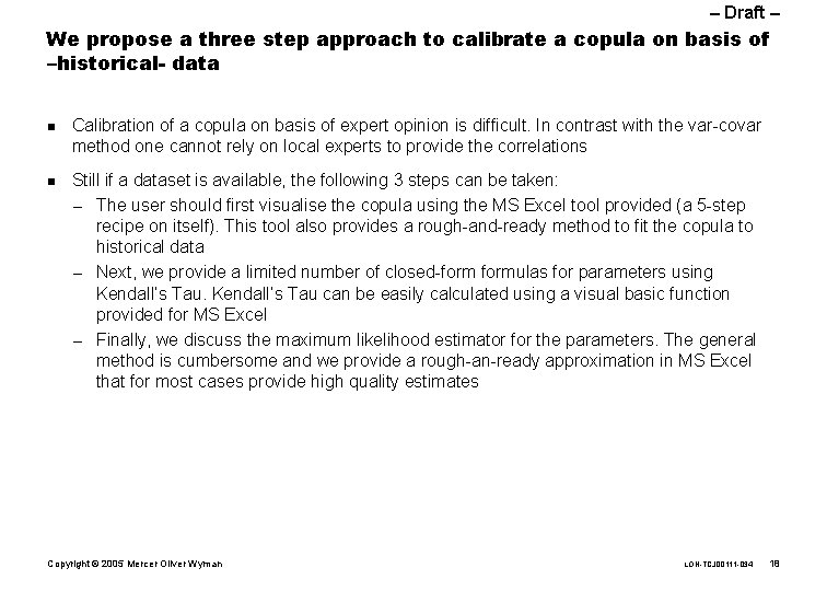
– Draft – We propose a three step approach to calibrate a copula on basis of –historical- data n n Calibration of a copula on basis of expert opinion is difficult. In contrast with the var-covar method one cannot rely on local experts to provide the correlations Still if a dataset is available, the following 3 steps can be taken: – The user should first visualise the copula using the MS Excel tool provided (a 5 -step recipe on itself). This tool also provides a rough-and-ready method to fit the copula to historical data – Next, we provide a limited number of closed-formulas for parameters using Kendall’s Tau can be easily calculated using a visual basic function provided for MS Excel – Finally, we discuss the maximum likelihood estimator for the parameters. The general method is cumbersome and we provide a rough-an-ready approximation in MS Excel that for most cases provide high quality estimates Copyright © 2005 Mercer Oliver Wyman LON-TCJ 00111 -034 18

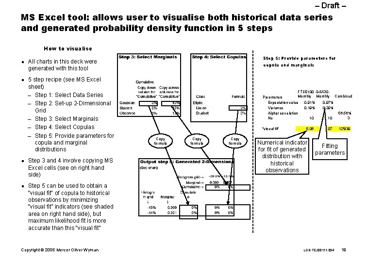
– Draft – MS Excel tool: allows user to visualise both historical data series and generated probability density function in 5 steps How to visualise n n Step 5: Provide parameters for All charts in this deck were generated with this tool 5 step recipe (see MS Excel sheet) – Step 1: Select Data Series – Step 2: Set-up 2 -Dimensional Grid – Step 3: Select Marginals – Step 4: Select Copulas – Step 5: Provide parameters for copula and marginal distributions Step 3 and 4 involve copying MS Excel cells (see on right hand side) copula and marginals FTSE 100 -DAX 30 Monthly Combined Parameters Expectation value 0. 91% 0. 97% Variance 0. 19% 0. 29% Alpha/ correlation 56. 56% Nu 10 10 3 "visual fit" Copy formula 5. 06 Numerical indicator fit of generated distribution with historical observations 3. 07 12'839 Fitting parameters Step 5 can be used to obtain a “visual fit“ of copula to historical observations by minimizing “visual fit” indicators (see shaded area on right hand side), but maximum likelihood fit is more accurate than this “visual fit” Copyright © 2005 Mercer Oliver Wyman LON-TCJ 00111 -034 19

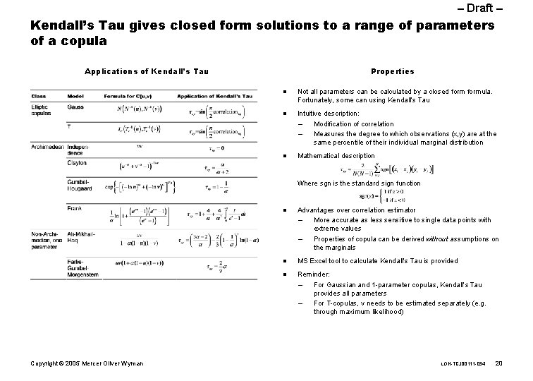
– Draft – Kendall’s Tau gives closed form solutions to a range of parameters of a copula Properties Applications of Kendall’s Tau n Not all parameters can be calculated by a closed formula. Fortunately, some can using Kendall’s Tau n Intuitive description: – Modification of correlation – Measures the degree to which observations (x, y) are at the same percentile of their individual marginal distribution n Mathematical description Where sgn is the standard sign function Copyright © 2005 Mercer Oliver Wyman n Advantages over correlation estimator – More accurate as less sensitive to single data points with extreme values – Properties of copula can be derived without assumptions on the marginals n MS Excel tool to calculate Kendall’s Tau is provided n Reminder: – For Gaussian and 1 -parameter copulas, Kendall’s Tau provides all parameters – For T-copulas, v needs to be estimated separately (e. g. through maximum likelihood) LON-TCJ 00111 -034 20

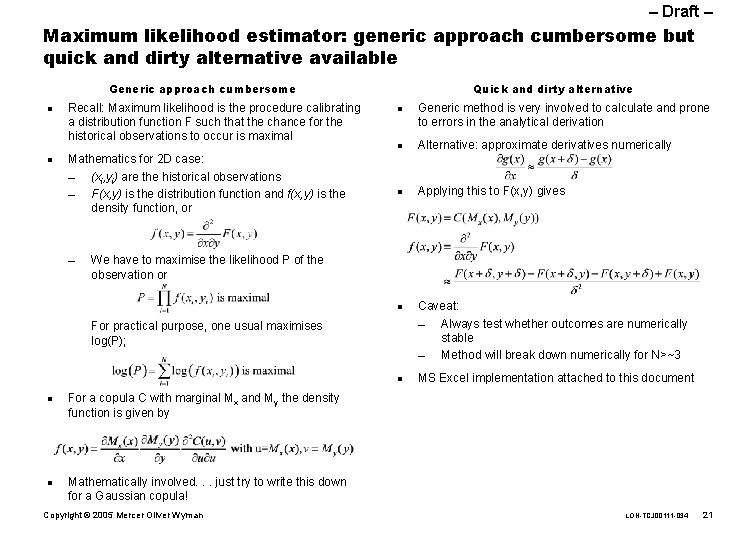
– Draft – Maximum likelihood estimator: generic approach cumbersome but quick and dirty alternative available Generic approach cumbersome n n Recall: Maximum likelihood is the procedure calibrating a distribution function F such that the chance for the historical observations to occur is maximal Mathematics for 2 D case: – (xi, yi) are the historical observations – F(x, y) is the distribution function and f(x, y) is the density function, or – Quick and dirty alternative n n Alternative: approximate derivatives numerically n Applying this to F(x, y) gives We have to maximise the likelihood P of the observation or n For practical purpose, one usual maximises log(P); n n n Generic method is very involved to calculate and prone to errors in the analytical derivation Caveat: – Always test whether outcomes are numerically stable – Method will break down numerically for N>~3 MS Excel implementation attached to this document For a copula C with marginal Mx and My the density function is given by Mathematically involved. . . just try to write this down for a Gaussian copula! Copyright © 2005 Mercer Oliver Wyman LON-TCJ 00111 -034 21

– Draft – Section 5 Sampling a copula Copyright © 2005 Mercer Oliver Wyman LON-TCJ 00111 -034 22

– Draft – We provide ready to use samplers in MS Excel for the Gaussian and T-copula n n n Sampling of a given distribution function means stochastically generating sets of observations for this distribution function Typical applications are found in pricing reinsurance contracts and in setting economic capital requirements A multivariate distribution function can always be expressed as the combination of a set of marginal distribution functions and a copula; this change of representation can fairly easily be implemented in an asset generator The generic algorithm to sample the copula representation of a multivariate distribution function is cumbersome For Gaussian, T and Archimedean copulas, there exist simple alternative algorithms. We provide an implementation in MS Excel for the algorithms of Gaussian and T-copulas All algorithms only sample the copula irrespective of the used marginal distribution functions; the observables are derived by inverting the marginal distribution functions Copyright © 2005 Mercer Oliver Wyman LON-TCJ 00111 -034 23

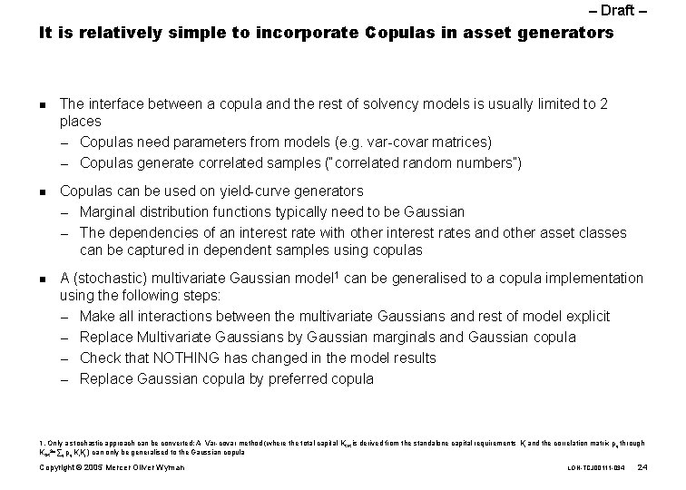
– Draft – It is relatively simple to incorporate Copulas in asset generators n n n The interface between a copula and the rest of solvency models is usually limited to 2 places – Copulas need parameters from models (e. g. var-covar matrices) – Copulas generate correlated samples (“correlated random numbers”) Copulas can be used on yield-curve generators – Marginal distribution functions typically need to be Gaussian – The dependencies of an interest rate with other interest rates and other asset classes can be captured in dependent samples using copulas A (stochastic) multivariate Gaussian model 1 can be generalised to a copula implementation using the following steps: – Make all interactions between the multivariate Gaussians and rest of model explicit – Replace Multivariate Gaussians by Gaussian marginals and Gaussian copula – Check that NOTHING has changed in the model results – Replace Gaussian copula by preferred copula 1. Only a stochastic approach can be converted; A Var-covar method (where the total capital Ktot is derived from the standalone capital requirements Ki and the correlation matrix ρij through Ktot 2=∑ij ρij Ki. Kj ) can only be generalised to the Gaussian copula Copyright © 2005 Mercer Oliver Wyman LON-TCJ 00111 -034 24

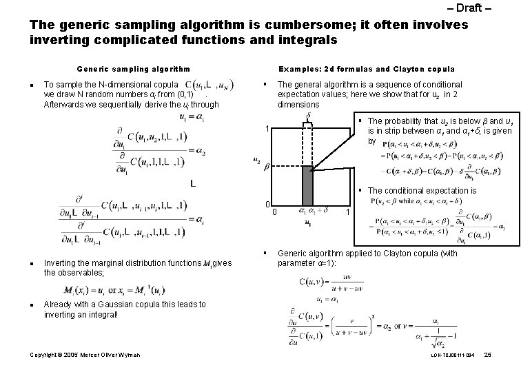
– Draft – The generic sampling algorithm is cumbersome; it often involves inverting complicated functions and integrals Generic sampling algorithm n Examples: 2 d formulas and Clayton copula To sample the N-dimensional copula we draw N random numbers αi from (0, 1). Afterwards we sequentially derive the ui through § The general algorithm is a sequence of conditional expectation values; here we show that for u 2 in 2 dimensions § The probability that u 2 is below β and u 1 is in strip between α 1 and α 1+δ, is given by 1 § The conditional expectation is 0 § n n Inverting the marginal distribution functions the observables; gives 0 1 Generic algorithm applied to Clayton copula (with parameter α=1): Already with a Gaussian copula this leads to inverting an integral! Copyright © 2005 Mercer Oliver Wyman LON-TCJ 00111 -034 25

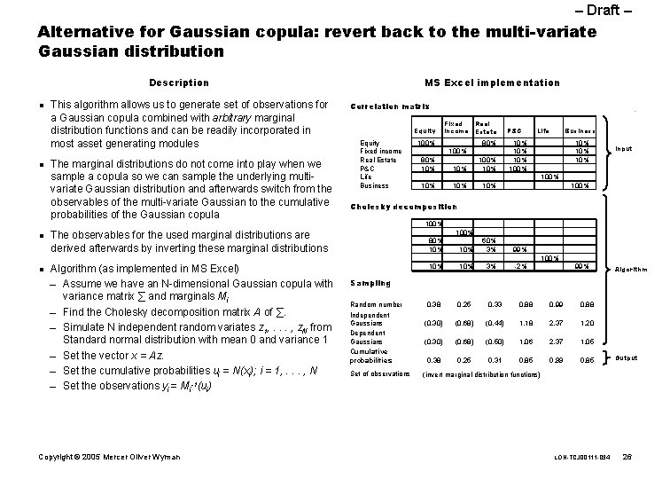
– Draft – Alternative for Gaussian copula: revert back to the multi-variate Gaussian distribution Description n n This algorithm allows us to generate set of observations for a Gaussian copula combined with arbitrary marginal distribution functions and can be readily incorporated in most asset generating modules The marginal distributions do not come into play when we sample a copula so we can sample the underlying multivariate Gaussian distribution and afterwards switch from the observables of the multi-variate Gaussian to the cumulative probabilities of the Gaussian copula MS Excel implementation Correlation matrix Equity Fixed income Real Estate P&C Life Business Copyright © 2005 Mercer Oliver Wyman P&C Life Business 100% 0% 80% 10% 0% 100% 0% 10% 80% 0% 10% 10% 100% 0% 100% 0% 10% 10% 0% 0% 100% Input Cholesky decomposition The observables for the used marginal distributions are derived afterwards by inverting these marginal distributions Algorithm (as implemented in MS Excel) – Assume we have an N-dimensional Gaussian copula with variance matrix ∑ and marginals Mi – Find the Cholesky decomposition matrix A of ∑. – Simulate N independent random variates z 1, . . . , z. N from Standard normal distribution with mean 0 and variance 1 – Set the vector x = Az. – Set the cumulative probabilities ui = N(xi); i = 1, . . . , N – Set the observations yi = Mi-1(ui) Fixed Real income Estate 100% 0% 80% 10% 0% 100% 0% 10% 0% 0% 60% 3% 0% 0% 0% 99% 0% 0% 100% -2% 0% 0% 0% 99% 0. 38 0. 25 0. 33 0. 88 0. 99 0. 88 (0. 30) (0. 68) (0. 44) 1. 18 2. 37 1. 20 (0. 30) (0. 68) (0. 50) 1. 06 2. 37 1. 05 0. 38 0. 25 0. 31 0. 85 0. 99 0. 85 Algorithm Sampling Random number Independent Gaussians Dependent Gaussians Cumulative probabilities Set of observations Output (invert marginal distribution functions) LON-TCJ 00111 -034 26

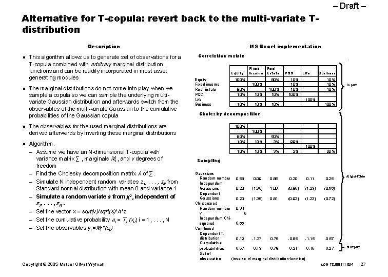
– Draft – Alternative for T-copula: revert back to the multi-variate Tdistribution Description n n This algorithm allows us to generate set of observations for a T-copula combined with arbitrary marginal distribution functions and can be readily incorporated in most asset generating modules The marginal distributions do not come into play when we sample a copula so we can sample the underlying multivariate Gaussian distribution and afterwards switch from the observables of the multi-variate Gaussian to the cumulative probabilities of the Gaussian copula MS Excel implementation Correlation matrix Equity Fixed income Real Estate P&C Life Business Copyright © 2005 Mercer Oliver Wyman 0% 80% 100% 0% 0% 10% 10% 0% 0% 10% P&C Life Business 10% 10% 100% 0% 100% 0% 10% 10% 0% 0% 100% 0% 99% 0% -2% 0% 0% 100% 0% 99% Input Cholesky decomposition The observables for the used marginal distributions are derived afterwards by inverting these marginal distributions Algorithm. – Assume we have an N-dimensional T-copula with variance matrix ∑ , marginals Mi , and v degrees of freedom – Find the Cholesky decomposition matrix A of ∑. – Simulate N independent random variates z 1, . . . , z. N from Standard normal distribution with mean 0 and variance 1 – Simulate a random variate s from χ2 v independent of z 1, . . . , z. N. – Set the vector x = sqrt(v)/sqrt(s)*A*z. – Set the cumulative probability ui = Tv (xi); i = 1, . . . , N – Set the observables yi =Mi-1(ui) 100% 0% 80% 10% Fixed Real income Estate 100% 0% 80% 10% 0% 100% 0% 10% 0% 0% 60% 3% Sampling Gaussians Random number 0. 58 0. 09 0. 86 0. 20 0. 11 Independent Gaussians 0. 20 (1. 35) 1. 09 (0. 85) (1. 23) Dependent Gaussians 0. 20 (1. 35) 0. 81 (0. 92) (1. 23) Chi-squared Random number 0. 34 v 5 Independent Chisquared 5. 66 Combined Dependent Tdistribution 0. 19 -1. 27 0. 76 -0. 86 -1. 16 Cumulative probabilities 0. 57 0. 13 0. 76 0. 21 0. 15 Set of observation (inverse of marginal distribution function) 0. 25 Algorithm (0. 66) (0. 72) -0. 67 0. 27 Output LON-TCJ 00111 -034 27

– Draft – Section 6 Further considerations on tail dependencies Copyright © 2005 Mercer Oliver Wyman LON-TCJ 00111 -034 28

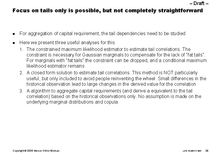
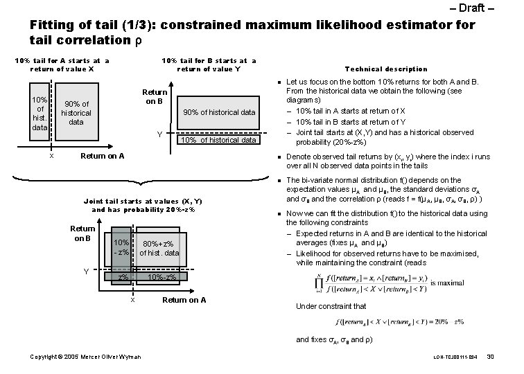
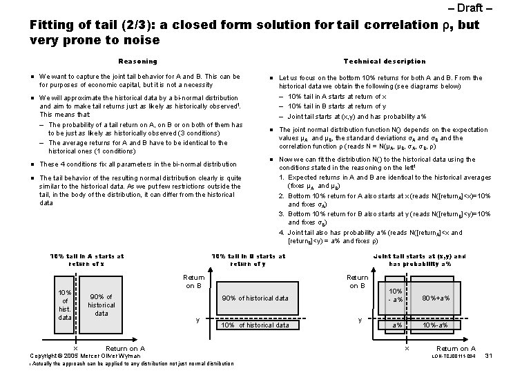
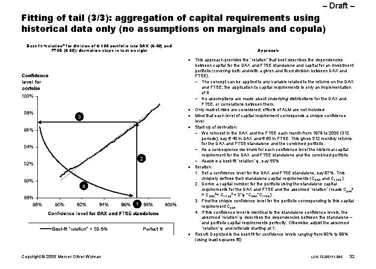
– Draft – Focus on tails only is possible, but not completely straightforward n n For aggregation of capital requirement, the tail dependencies need to be studied Here we present three useful analyses for this 1. The constrained maximum likelihood estimator to estimate tail correlations. The constraint is necessary for Gaussian marginals to compensate for the lack of “fat tails”. For marginals with “fat tails” the constraint can be dropped, and a conditional maximum likelihood estimator remains 2. A closed form solution to estimate tail correlations. This method is NOT particularly useful, but only included to avoid people reinventing the wheel. Small differences in the historical observation lead to large changes in the derived value for the correlation 3. A algorithm to aggregate capital requirements (and derive a equivalent to the tail correlation) based on the historical observations only. No assumption is made on the underlying marginal distributions and copula Copyright © 2005 Mercer Oliver Wyman LON-TCJ 00111 -034 29

– Draft – Fitting of tail (1/3): constrained maximum likelihood estimator for tail correlation ρ 10% tail for A starts at a return of value X 10% tail for B starts at a return of value Y Technical description n 10% of hist. data Return on B 90% of historical data Y x 10% of historical data Return on A n n Joint tail starts at values (X, Y) and has probability 20%-z% Return on B Y 10% - z% 80%+z% of hist. data z% n Let us focus on the bottom 10% returns for both A and B. From the historical data we obtain the following (see diagrams) – 10% tail in A starts at return of X – 10% tail in B starts at return of Y – Joint tail starts at (X, Y) and has a historical observed probability (20%-z%) Denote observed tail returns by (xi, yi) where the index i runs over all N observed data points in the tails The bi-variate normal distribution f() depends on the expectation values µA and µB, the standard deviations σA and σB and the correlation ρ (reads f = f(µA, µB, σA, σB, ρ) ) Now we can fit the distribution f() to the historical data using the following constraints – Expected returns in A and B are identical to the historical averages (fixes µA and µB) – Likelihood for observed returns have to be maximised, while maintaining the constraint (reads 10%-z% x Return on A Under constraint that and fixes σA, σB and ρ) Copyright © 2005 Mercer Oliver Wyman LON-TCJ 00111 -034 30

– Draft – Fitting of tail (2/3): a closed form solution for tail correlation ρ, but very prone to noise Technical description Reasoning n We want to capture the joint tail behavior for A and B. This can be for purposes of economic capital, but it is not a necessity n We will approximate the historical data by a bi-normal distribution and aim to make tail returns just as likely as historically observed 1. This means that: – The probability of a tail return on A, on B or on both of them has to be just as likely as historically observed (3 conditions) – The average returns for A and B have to be identical to the historical ones (1 conditions) n These 4 conditions fix all parameters in the bi-normal distribution n The tail behavior of the resulting normal distribution clearly is quite similar to the historical data. As we put few restrictions outside the tail, in the body of the distribution, it can differ from the historical data 10% tail in A starts at return of x Let us focus on the bottom 10% returns for both A and B. From the historical data we obtain the following (see diagrams below) – 10% tail in A starts at return of x – 10% tail in B starts at return of y – Joint tail starts at (x, y) and has probability a% n The joint normal distribution function N() depends on the expectation values µA and µB, the standard deviations σA and σB and the correlation function ρ (reads N = N(µA, µB, σA, σB, ρ) n Now we can fit the distribution N() to the historical data using the conditions stated in the reasoning on the left 1 1. Expected returns in A and B are identical to the historical averages (fixes µA and µB) 2. Bottom 10% return for A also starts at x (reads N([return. A]<x)=10% and fixes σA) 3. Bottom 10% return for B also starts at y (reads N([return. B]<y)=10% and fixes σB) 4. Joint tail also has probability a% (reads N([return. A]<x and [return. B]<y) = a% and fixes ρ) 10% tail in B starts at return of y Return on B 10% of hist. data 90% of historical data x Joint tail starts at (x, y) and has probability a% Return on B 90% of historical data y 10% of historical data Return on A Copyright © 2005 Mercer Oliver Wyman 1. Actually n the approach can be applied to any distribution not just normal distribution y 10% - a% 80%+a% a% 10%-a% x Return on A LON-TCJ 00111 -034 31

– Draft – Fitting of tail (3/3): aggregation of capital requirements using historical data only (no assumptions on marginals and copula) Best-fit “relation” for division of € 100 portfolio into DAX (€ 40) and FTSE (€ 60); derivation steps in text on right Approach n n 3 n n 2 n 4 1 n Copyright © 2005 Mercer Oliver Wyman This approach provides the “relation” that best describes the dependencies between capital for the DAX and FTSE standalone and capital for an investment portfolio (covering both and with a given and fixed division between DAX and FTSE). – The concept can be applied to any variable related to the returns on the DAX and FTSE; the application to capital requirements is only an implementation of it – No assumptions are made about underlying distributions for the DAX and FTSE, or correlations between them. Only market risks are considered; effects of ALM are not included Mind that each level of capital requirement corresponds a unique confidence level Start-up of derivation: – We reinvest in the DAX and the FTSE each month from 1979 to 2005 (312 periods), say € 40 in DAX and € 60 in FTSE. This gives 312 monthly returns for the DAX and FTSE standalone and the combined portfolio. – As a consequence we know for each confidence level the historical capital requirement for the DAX and FTSE standalone and the combined portfolio – Assume a best-fit “relation” φ, say 55% Iteration: 1. Set a confidence level for the DAX and FTSE standalone, say 97%. This uniquely defines their standalone capital requirements (CDAX and CFTSE ) 2. Derive a capital number for the portfolio using the standalone capital requirements for the DAX and FTSE and the assumed “relation” (reads Cport 2 = CDAX 2+ CFTSE 2 + 2*φ *CDAX*CFTSE) 3. Find the unique confidence level for the portfolio corresponding to this capital requirement Cport 4. If this confidence level is identical to the standalone confidence levels, the assumed “relation” φ describes the dependencies between the standalone – and portfolio capital requirements perfectly. Otherwise adjust the assumed “relation” φ and reiterate starting at 1. Result: Depicted is the best-fit for confidence levels ranging from 90% to 99% (using least squares fit) LON-TCJ 00111 -034 32

– Draft – Section 5 References Copyright © 2005 Mercer Oliver Wyman LON-TCJ 00111 -034 33

– Draft – For other open questions we refer to the literature Copyright © 2005 Mercer Oliver Wyman LON-TCJ 00111 -034 34

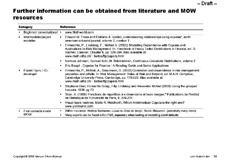
– Draft – Further information can be obtained from literature and MOW resources Copyright © 2005 Mercer Oliver Wyman LON-TCJ 00111 -034 35