12 Graphs and Trees 2 Summary Aaron Tan

12. Graphs and Trees 2 Summary Aaron Tan 5 – 9 November 2018 1

Summary 12. Graphs and Trees 2 10. 5 Trees • Definitions: circuit-free, trivial tree, forest • Characterizing trees: terminal vertex (leaf), internal vertex 10. 6 Rooted Trees • Definitions: rooted tree, root, level, height, child, parent, sibling, ancestor, descendant • Definitions: binary tree, full binary tree, subtree • Binary tree traversal: breadth-first-search (BFD), depth-first-search (DFS) 10. 7 Spanning Trees and Shortest Paths • Definitions: spanning tree, weighted graph, minimum spanning tree (MST) • Kruskal’s algorithm, Prim’s algorithm • Dijkstra’s shortest path algorithm 2

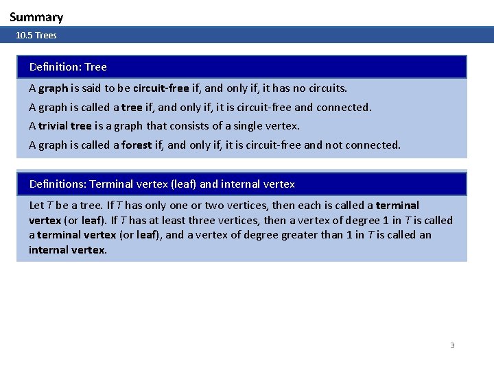
Summary 10. 5 Trees Definition: Tree A graph is said to be circuit-free if, and only if, it has no circuits. A graph is called a tree if, and only if, it is circuit-free and connected. A trivial tree is a graph that consists of a single vertex. A graph is called a forest if, and only if, it is circuit-free and not connected. Definitions: Terminal vertex (leaf) and internal vertex Let T be a tree. If T has only one or two vertices, then each is called a terminal vertex (or leaf). If T has at least three vertices, then a vertex of degree 1 in T is called a terminal vertex (or leaf), and a vertex of degree greater than 1 in T is called an internal vertex. 3

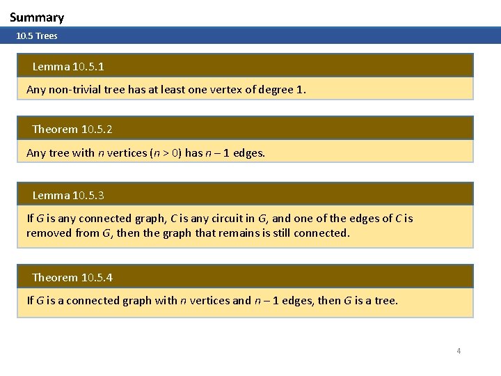
Summary 10. 5 Trees Lemma 10. 5. 1 Any non-trivial tree has at least one vertex of degree 1. Theorem 10. 5. 2 Any tree with n vertices (n > 0) has n – 1 edges. Lemma 10. 5. 3 If G is any connected graph, C is any circuit in G, and one of the edges of C is removed from G, then the graph that remains is still connected. Theorem 10. 5. 4 If G is a connected graph with n vertices and n – 1 edges, then G is a tree. 4

Summary 10. 6 Rooted Trees Definitions: Rooted Tree, Level, Height A rooted tree is a tree in which there is one vertex that is distinguished from the others and is called the root. The level of a vertex is the number of edges along the unique path between it and the root. The height of a rooted tree is the maximum level of any vertex of the tree. Definitions: Child, Parent, Sibling, Ancestor, Descendant Given the root or any internal vertex v of a rooted tree, the children of v are all those vertices that are adjacent to v and are one level farther away from the root than v. If w is a child of v, then v is called the parent of w, and two distinct vertices that are both children of the same parent are called siblings. Given two distinct vertices v and w, if v lies on the unique path between w and the root, then v is an ancestor of w, and w is a descendant of v. 5

Summary 10. 6 Rooted Trees Definitions: Binary Tree, Full Binary Tree A binary tree is a rooted tree in which every parent has at most two children. Each child is designated either a left child or a right child (but not both), and every parent has at most one left child and one right child. A full binary tree is a binary tree in which each parent has exactly two children. Definitions: Left Subtree, Right Subtree Given any parent v in a binary tree T, if v has a left child, then the left subtree of v is the binary tree whose root is the left child of v, whose vertices consist of the left child of v and all its descendants, and whose edges consist of all those edges of T that connect the vertices of the left subtree. The right subtree of v is defined analogously. 6

Summary 10. 6 Rooted Trees Theorem 10. 6. 1: Full Binary Tree Theorem If T is a full binary tree with k internal vertices, then T has a total of 2 k + 1 vertices and has k + 1 terminal vertices (leaves). Theorem 10. 6. 2 For non-negative integers h, if T is any binary tree with height h and t terminal vertices (leaves), then t 2 h Equivalently, log 2 t h 7

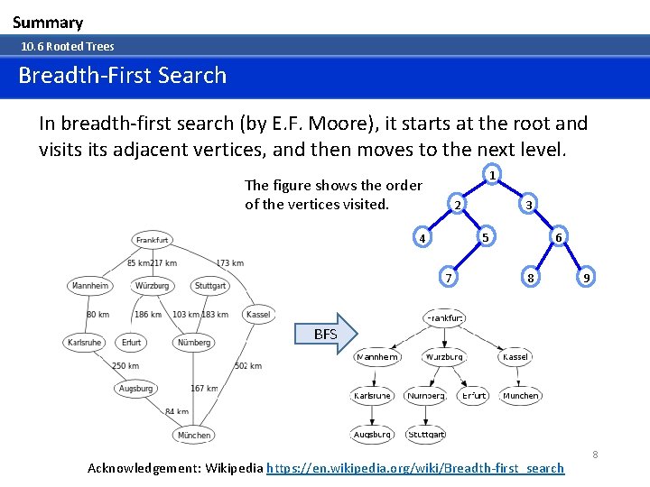
Summary 10. 6 Rooted Trees Breadth-First Search In breadth-first search (by E. F. Moore), it starts at the root and visits adjacent vertices, and then moves to the next level. 1 The figure shows the order of the vertices visited. 2 3 5 4 7 6 8 9 BFS Acknowledgement: Wikipedia https: //en. wikipedia. org/wiki/Breadth-first_search 8

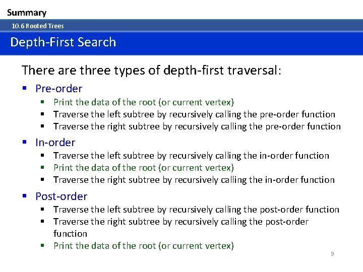
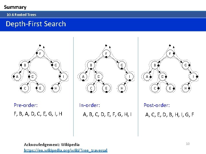
Summary 10. 6 Rooted Trees Depth-First Search There are three types of depth-first traversal: § Pre-order § Print the data of the root (or current vertex) § Traverse the left subtree by recursively calling the pre-order function § Traverse the right subtree by recursively calling the pre-order function § In-order § Traverse the left subtree by recursively calling the in-order function § Print the data of the root (or current vertex) § Traverse the right subtree by recursively calling the in-order function § Post-order § Traverse the left subtree by recursively calling the post-order function § Traverse the right subtree by recursively calling the post-order function § Print the data of the root (or current vertex) 9

Summary 10. 6 Rooted Trees Depth-First Search Pre-order: F, B, A, D, C, E, G, I, H In-order: A, B, C, D, E, F, G, H, I Acknowledgement: Wikipedia https: //en. wikipedia. org/wiki/Tree_traversal Post-order: A, C, E, D, B, H, I, G, F 10

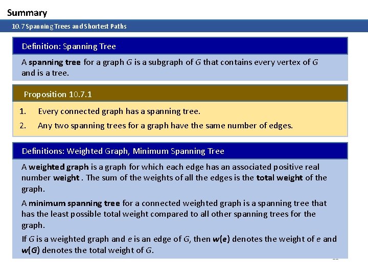
Summary 10. 7 Spanning Trees and Shortest Paths Definition: Spanning Tree A spanning tree for a graph G is a subgraph of G that contains every vertex of G and is a tree. Proposition 10. 7. 1 1. 2. Every connected graph has a spanning tree. Any two spanning trees for a graph have the same number of edges. Definitions: Weighted Graph, Minimum Spanning Tree A weighted graph is a graph for which each edge has an associated positive real number weight. The sum of the weights of all the edges is the total weight of the graph. A minimum spanning tree for a connected weighted graph is a spanning tree that has the least possible total weight compared to all other spanning trees for the graph. If G is a weighted graph and e is an edge of G, then w(e) denotes the weight of e and w(G) denotes the total weight of G. 11

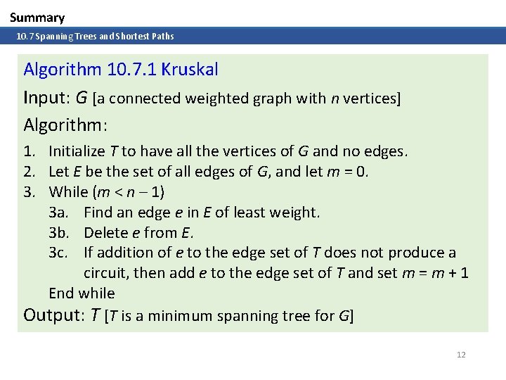
Summary 10. 7 Spanning Trees and Shortest Paths Algorithm 10. 7. 1 Kruskal Input: G [a connected weighted graph with n vertices] Algorithm: 1. Initialize T to have all the vertices of G and no edges. 2. Let E be the set of all edges of G, and let m = 0. 3. While (m < n – 1) 3 a. Find an edge e in E of least weight. 3 b. Delete e from E. 3 c. If addition of e to the edge set of T does not produce a circuit, then add e to the edge set of T and set m = m + 1 End while Output: T [T is a minimum spanning tree for G] 12

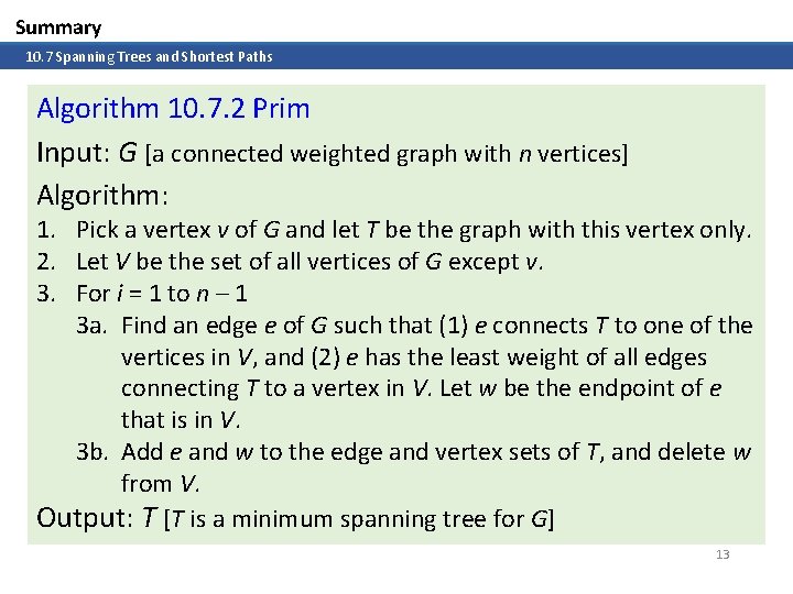
Summary 10. 7 Spanning Trees and Shortest Paths Algorithm 10. 7. 2 Prim Input: G [a connected weighted graph with n vertices] Algorithm: 1. Pick a vertex v of G and let T be the graph with this vertex only. 2. Let V be the set of all vertices of G except v. 3. For i = 1 to n – 1 3 a. Find an edge e of G such that (1) e connects T to one of the vertices in V, and (2) e has the least weight of all edges connecting T to a vertex in V. Let w be the endpoint of e that is in V. 3 b. Add e and w to the edge and vertex sets of T, and delete w from V. Output: T [T is a minimum spanning tree for G] 13

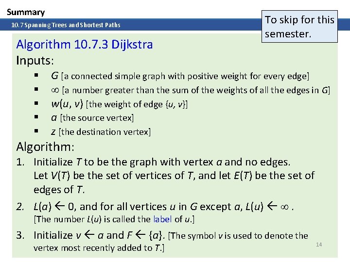
Summary 10. 7 Spanning Trees and Shortest Paths Algorithm 10. 7. 3 Dijkstra Inputs: § § § To skip for this semester. G [a connected simple graph with positive weight for every edge] [a number greater than the sum of the weights of all the edges in G] w(u, v) [the weight of edge {u, v}] a [the source vertex] z [the destination vertex] Algorithm: 1. Initialize T to be the graph with vertex a and no edges. Let V(T) be the set of vertices of T, and let E(T) be the set of edges of T. 2. L(a) 0, and for all vertices u in G except a, L(u) . [The number L(u) is called the label of u. ] 3. Initialize v a and F {a}. [The symbol v is used to denote the vertex most recently added to T. ] 14

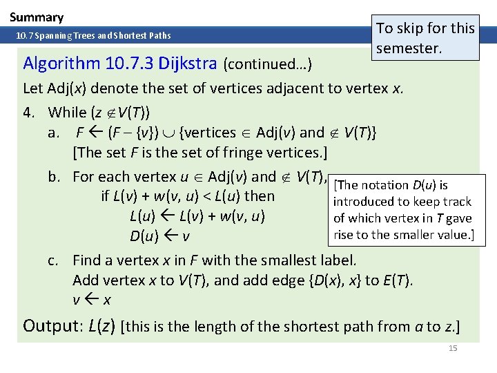
Summary 10. 7 Spanning Trees and Shortest Paths Algorithm 10. 7. 3 Dijkstra (continued…) To skip for this semester. Let Adj(x) denote the set of vertices adjacent to vertex x. 4. While (z V(T)) a. F (F – {v}) {vertices Adj(v) and V(T)} [The set F is the set of fringe vertices. ] b. For each vertex u Adj(v) and V(T), [The notation D(u) is if L(v) + w(v, u) < L(u) then introduced to keep track L(u) L(v) + w(v, u) of which vertex in T gave rise to the smaller value. ] D(u) v c. Find a vertex x in F with the smallest label. Add vertex x to V(T), and add edge {D(x), x} to E(T). v x Output: L(z) [this is the length of the shortest path from a to z. ] 15

END OF FILE 16