1 Carrier concentrations and current LECTURE 6 Density

1 Carrier concentrations and current LECTURE 6 • Density of states • Carrier concentrations at equilibrium • Maxwellians and hemi-Maxwellians • Current and energy gradients • Diffusion current • Drift current

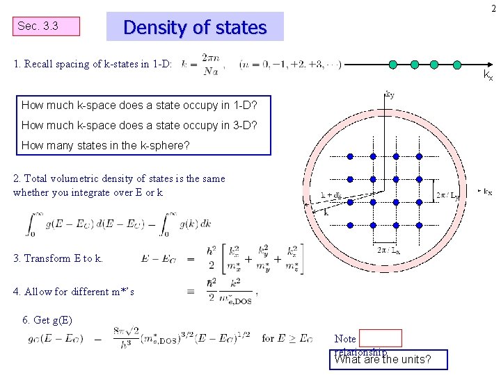
2 Sec. 3. 3 Density of states 1. Recall spacing of k-states in 1 -D: kx How much k-space does a state occupy in 1 -D? How much k-space does a state occupy in 3 -D? How many states in the k-sphere? 2. Total volumetric density of states is the same whether you integrate over E or k 3. Transform E to k. 4. Allow for different m*’s 6. Get g(E) Note parabolic relationship What are the units?

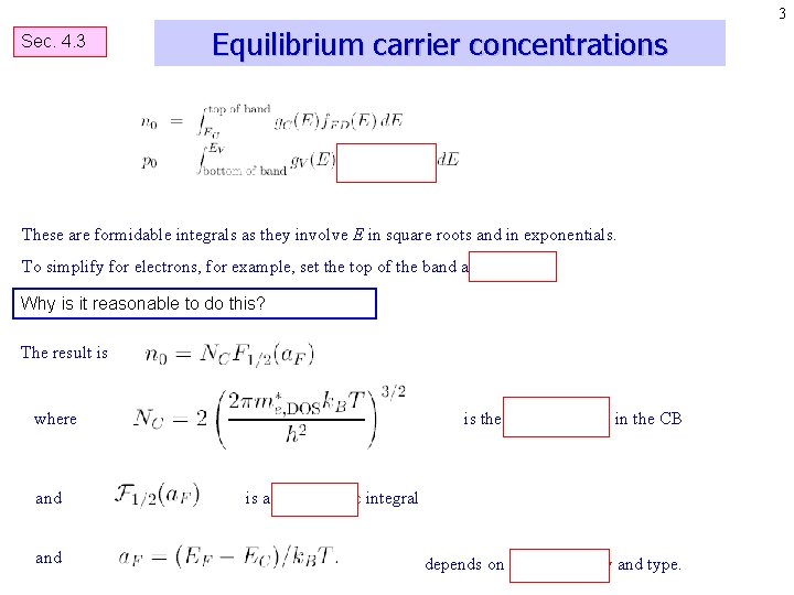
3 Sec. 4. 3 Equilibrium carrier concentrations These are formidable integrals as they involve E in square roots and in exponentials. To simplify for electrons, for example, set the top of the band at infinity. Why is it reasonable to do this? The result is where and is the Effective DOS in the CB is a Fermi-Dirac integral depends on doping density and type.

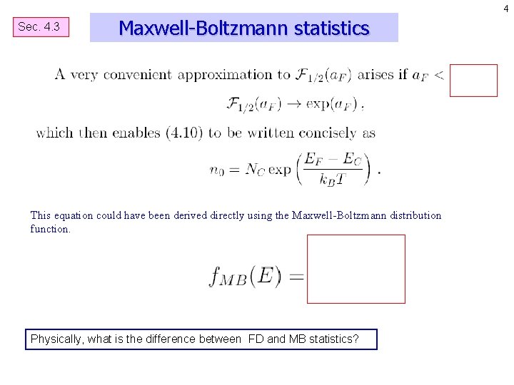
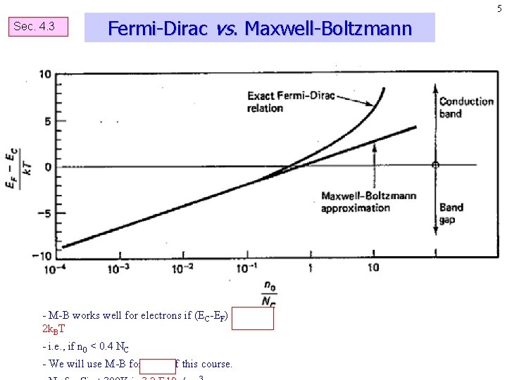
4 Sec. 4. 3 Maxwell-Boltzmann statistics This equation could have been derived directly using the Maxwell-Boltzmann distribution function. Physically, what is the difference between FD and MB statistics?

5 Sec. 4. 3 Fermi-Dirac vs. Maxwell-Boltzmann - M-B works well for electrons if (EC-EF) > 2 k. BT - i. e. , if n 0 < 0. 4 NC - We will use M-B for most of this course.

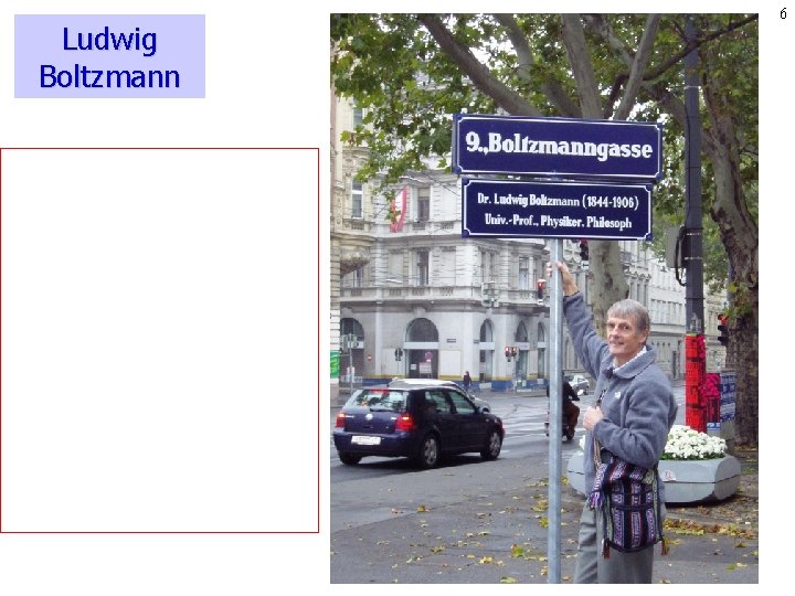
Ludwig Boltzmann 6

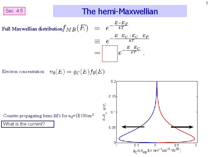
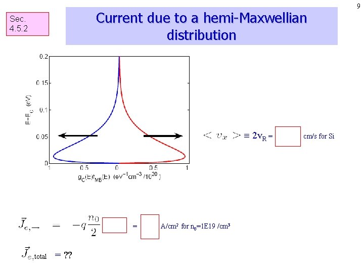
7 Sec. 4. 5 The hemi-Maxwellian Full Maxwellian distribution Electron concentration Counter-propagating hemi-M's for n 0=1 E 19/cm 3 What is the current?

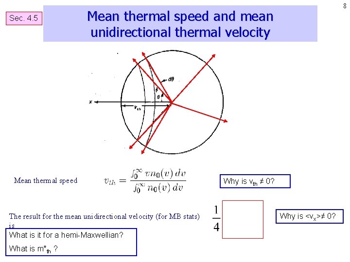
Sec. 4. 5 Mean thermal speed and mean unidirectional thermal velocity Mean thermal speed The result for the mean unidirectional velocity (for MB stats) is What is it for a hemi-Maxwellian? What is m*th ? 8 Why is vth ≠ 0? Why is <vx>≠ 0?

Current due to a hemi-Maxwellian distribution Sec. 4. 5. 2 2 v. R = = 8 E 6 total = ? ? A/cm 2 for n 0=1 E 19 /cm 3 1. 06 E 7 cm/s for Si 9

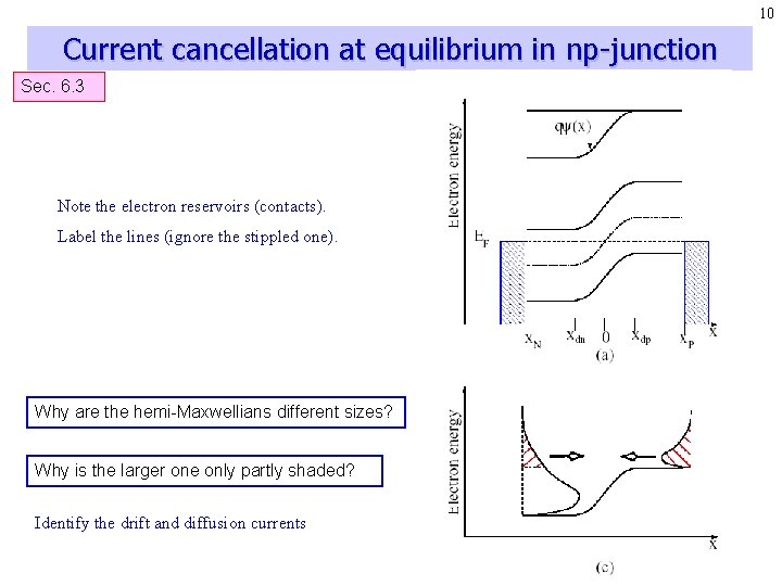
10 Current cancellation at equilibrium in np-junction Sec. 6. 3 Note the electron reservoirs (contacts). Label the lines (ignore the stippled one). Why are the hemi-Maxwellians different sizes? Why is the larger one only partly shaded? Identify the drift and diffusion currents

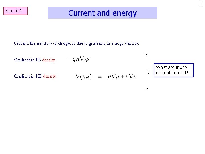
11 Sec. 5. 1 Current and energy Current, the net flow of charge, is due to gradients in energy density. Gradient in PE density Gradient in KE density What are these currents called?

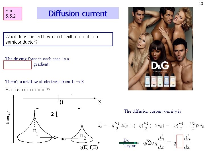
12 Sec. 5. 5. 2 Diffusion current What does this ad have to do with current in a semiconductor? The driving force in each case is a concentration gradient. There's a net flow of electrons from L R Energy Even at equilibrium ? ? The diffusion current density is 2 g(E) f(E) Do Taylor

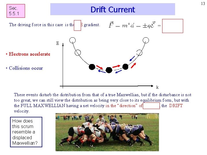
13 Drift Current Sec. 5. 5. 1 The driving force in this case is the PE gradient. E • Electrons accelerate • Collisions occur k These events disturb the distribution from that of a true Maxwellian, but if the disturbance is not too great, we can still view the distribution as being very close to its equilibrium form, but with the FULL MAXWELLIAN having a net velocity in the “direction” of the field, the DRIFT velocity. How does this scrum resemble a displaced Maxwellian?

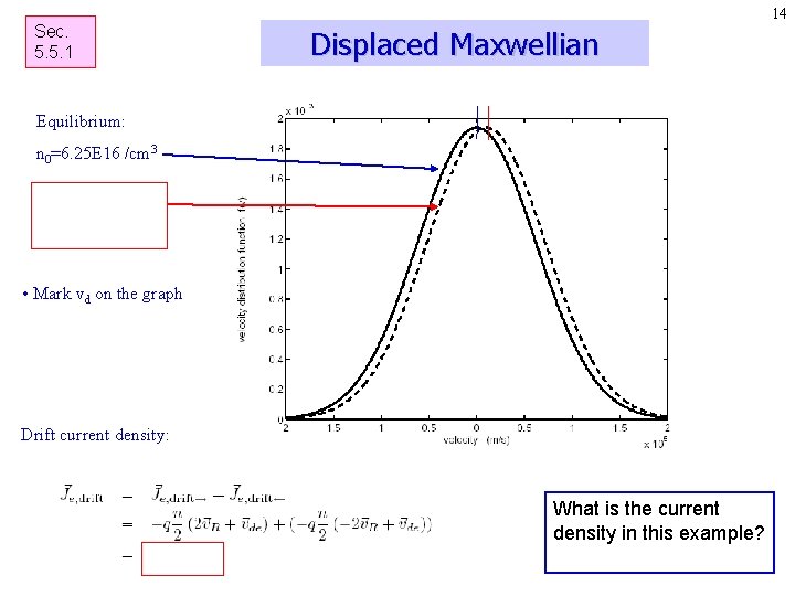
Sec. 5. 5. 1 14 Displaced Maxwellian Equilibrium: n 0=6. 25 E 16 /cm 3 n=6. 25 E 16 /cm 3 vd=2 v. R/10 • Mark vd on the graph Drift current density: What is the current density in this example?