Utility Theory Types of utility theories Six Types

Utility Theory

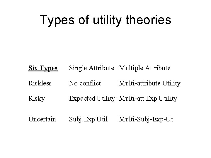
Types of utility theories Six Types Single Attribute Multiple Attribute Riskless No conflict Risky Expected Utility Multi-att Exp Utility Uncertain Subj Exp Util Multi-attribute Utility Multi-Subj-Exp-Ut

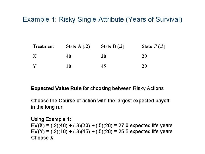
Example 1: Risky Single-Attribute (Years of Survival) Treatment State A (. 2) State B (. 3) State C (. 5) X 40 30 20 Y 10 45 20 Expected Value Rule for choosing between Risky Actions Choose the Course of action with the largest expected payoff in the long run Using Example 1: EV(X) = (. 2)(40) + (. 3)(30) + (. 5)(20) = 27. 0 expected life years EV(Y) = (. 2)(10) + (. 3)(45) + (. 5)(20) = 25. 5 expected life years Choose X

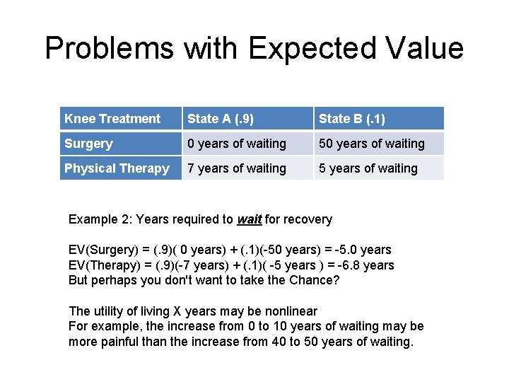
Problems with Expected Value Knee Treatment State A (. 9) State B (. 1) Surgery 0 years of waiting 50 years of waiting Physical Therapy 7 years of waiting 5 years of waiting Example 2: Years required to wait for recovery EV(Surgery) = (. 9)( 0 years) + (. 1)(-50 years) = -5. 0 years EV(Therapy) = (. 9)(-7 years) + (. 1)( -5 years ) = -6. 8 years But perhaps you don't want to take the Chance? The utility of living X years may be nonlinear For example, the increase from 0 to 10 years of waiting may be more painful than the increase from 40 to 50 years of waiting.

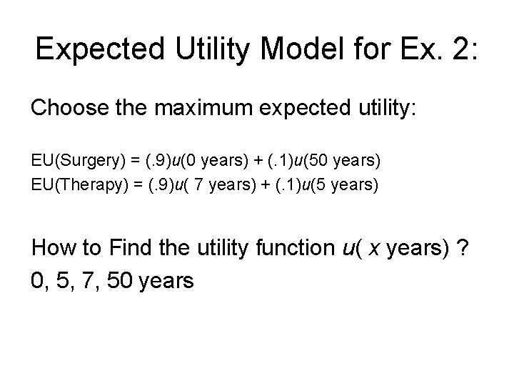
Expected Utility Model for Ex. 2: Choose the maximum expected utility: EU(Surgery) = (. 9)u(0 years) + (. 1)u(50 years) EU(Therapy) = (. 9)u( 7 years) + (. 1)u(5 years) How to Find the utility function u( x years) ? 0, 5, 7, 50 years

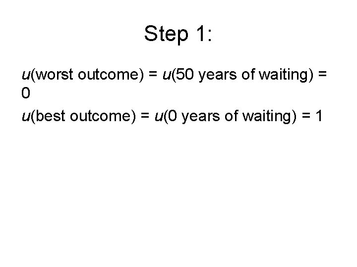
Step 1: u(worst outcome) = u(50 years of waiting) = 0 u(best outcome) = u(0 years of waiting) = 1

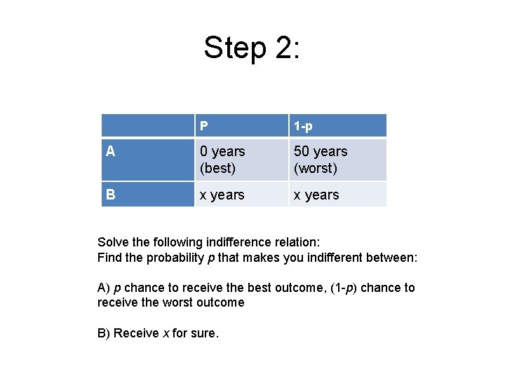
Step 2: P 1 -p A 0 years (best) 50 years (worst) B x years Solve the following indifference relation: Find the probability p that makes you indifferent between: A) p chance to receive the best outcome, (1 -p) chance to receive the worst outcome B) Receive x for sure.

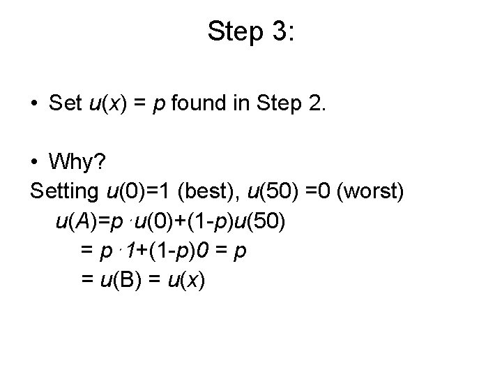
Step 3: • Set u(x) = p found in Step 2. • Why? Setting u(0)=1 (best), u(50) =0 (worst) u(A)=p⋅u(0)+(1 -p)u(50) = p⋅1+(1 -p)0 = p = u(B) = u(x)

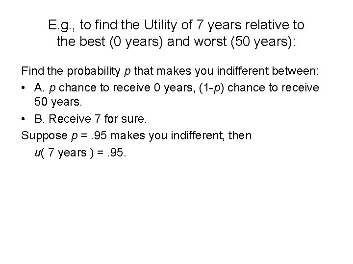
E. g. , to find the Utility of 7 years relative to the best (0 years) and worst (50 years): Find the probability p that makes you indifferent between: • A. p chance to receive 0 years, (1 -p) chance to receive 50 years. • B. Receive 7 for sure. Suppose p =. 95 makes you indifferent, then u( 7 years ) =. 95.

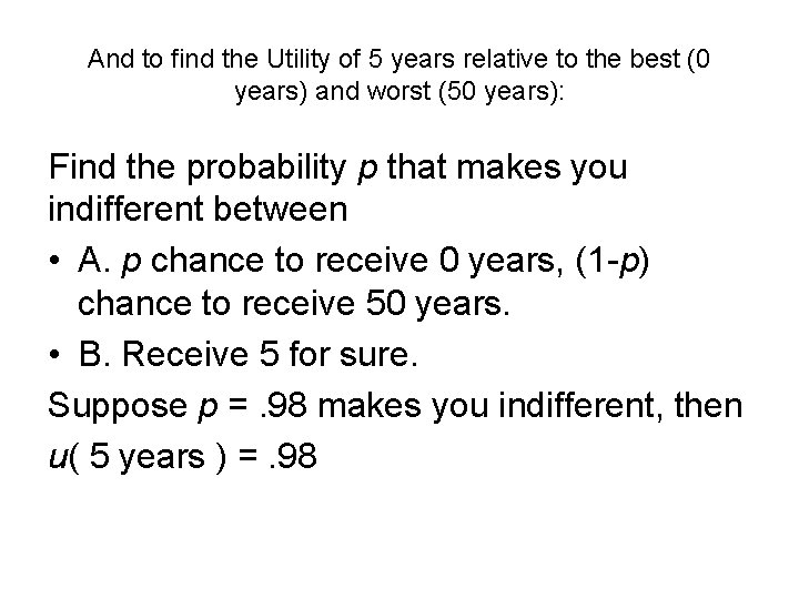
And to find the Utility of 5 years relative to the best (0 years) and worst (50 years): Find the probability p that makes you indifferent between • A. p chance to receive 0 years, (1 -p) chance to receive 50 years. • B. Receive 5 for sure. Suppose p =. 98 makes you indifferent, then u( 5 years ) =. 98

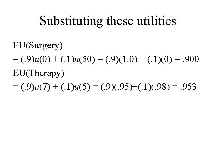
Substituting these utilities EU(Surgery) = (. 9)u(0) + (. 1)u(50) = (. 9)(1. 0) + (. 1)(0) =. 900 EU(Therapy) = (. 9)u(7) + (. 1)u(5) = (. 9)(. 95)+(. 1)(. 98) =. 953

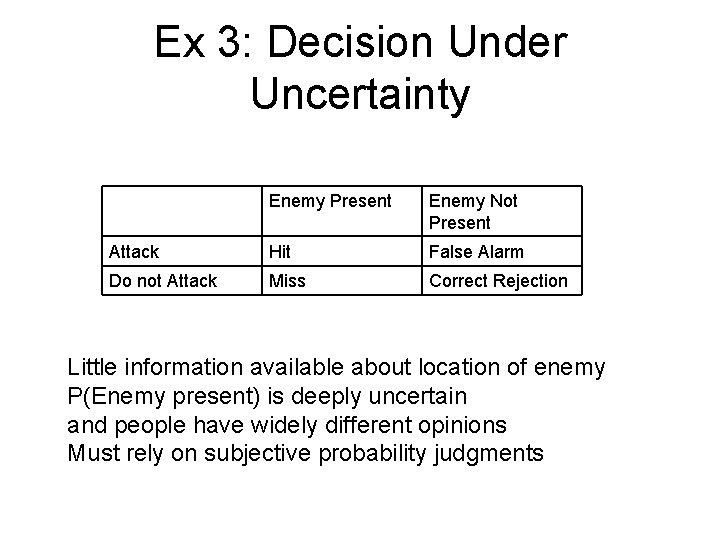
Ex 3: Decision Under Uncertainty Enemy Present Enemy Not Present Attack Hit False Alarm Do not Attack Miss Correct Rejection Little information available about location of enemy P(Enemy present) is deeply uncertain and people have widely different opinions Must rely on subjective probability judgments

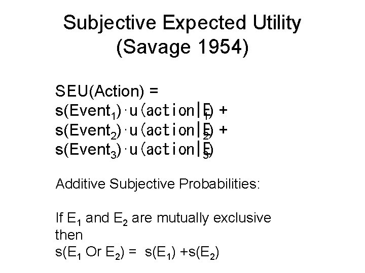
Subjective Expected Utility (Savage 1954) SEU(Action) = s(Event 1)⋅u(action|E 1) + s(Event 2)⋅u(action|E 2) + s(Event 3)⋅u(action|E 3) Additive Subjective Probabilities: If E 1 and E 2 are mutually exclusive then s(E 1 Or E 2) = s(E 1) +s(E 2)

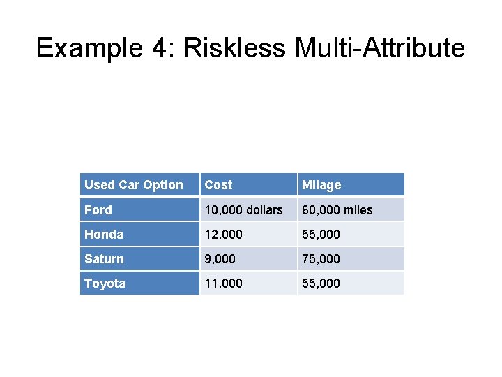
Example 4: Riskless Multi-Attribute Used Car Option Cost Milage Ford 10, 000 dollars 60, 000 miles Honda 12, 000 55, 000 Saturn 9, 000 75, 000 Toyota 11, 000 55, 000

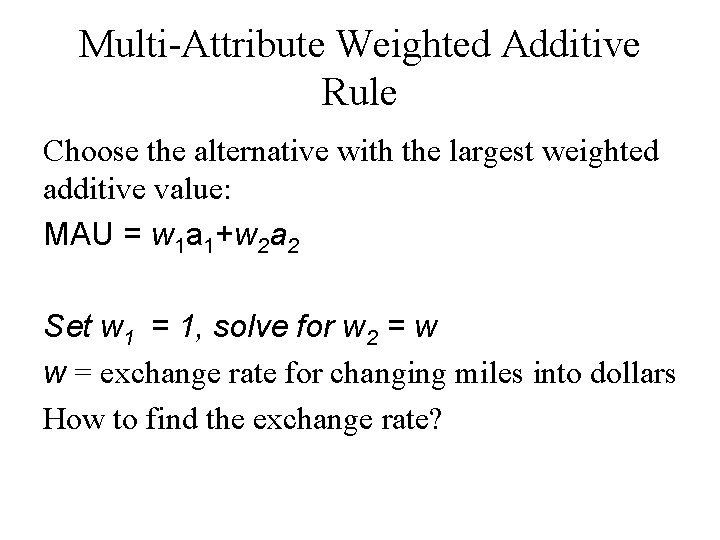
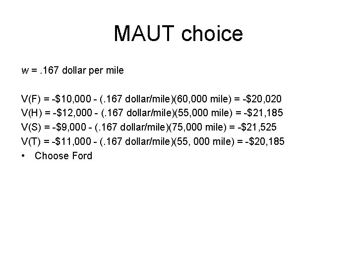
Multi-Attribute Weighted Additive Rule Choose the alternative with the largest weighted additive value: MAU = w 1 a 1+w 2 a 2 Set w 1 = 1, solve for w 2 = w w = exchange rate for changing miles into dollars How to find the exchange rate?

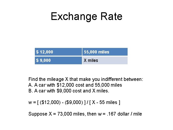
Exchange Rate $ 12, 000 55, 000 miles $ 9, 000 X miles Find the mileage X that make you indifferent between: A. A car with $12, 000 cost and 55, 000 miles B. A car with $9, 000 cost and X miles. w = [ ($12, 000) - ($9, 000) ] / [ X - 55 miles ] Suppose X = 73, 000 miles, then w =. 167 dollar / mile

MAUT choice w =. 167 dollar per mile V(F) = -$10, 000 - (. 167 dollar/mile)(60, 000 mile) = -$20, 020 V(H) = -$12, 000 - (. 167 dollar/mile)(55, 000 mile) = -$21, 185 V(S) = -$9, 000 - (. 167 dollar/mile)(75, 000 mile) = -$21, 525 V(T) = -$11, 000 - (. 167 dollar/mile)(55, 000 mile) = -$20, 185 • Choose Ford

Alternative Multi-attribute Models

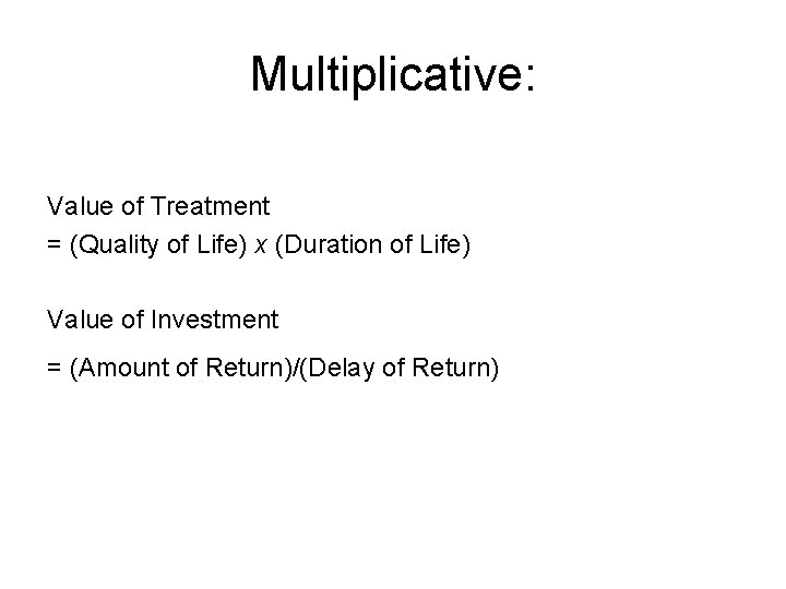
Multiplicative: Value of Treatment = (Quality of Life) x (Duration of Life) Value of Investment = (Amount of Return)/(Delay of Return)

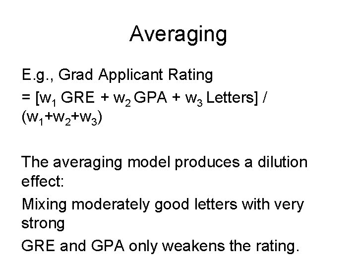
Averaging E. g. , Grad Applicant Rating = [w 1 GRE + w 2 GPA + w 3 Letters] / (w 1+w 2+w 3) The averaging model produces a dilution effect: Mixing moderately good letters with very strong GRE and GPA only weakens the rating.

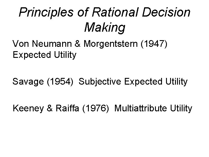
Principles of Rational Decision Making Von Neumann & Morgentstern (1947) Expected Utility Savage (1954) Subjective Expected Utility Keeney & Raiffa (1976) Multiattribute Utility

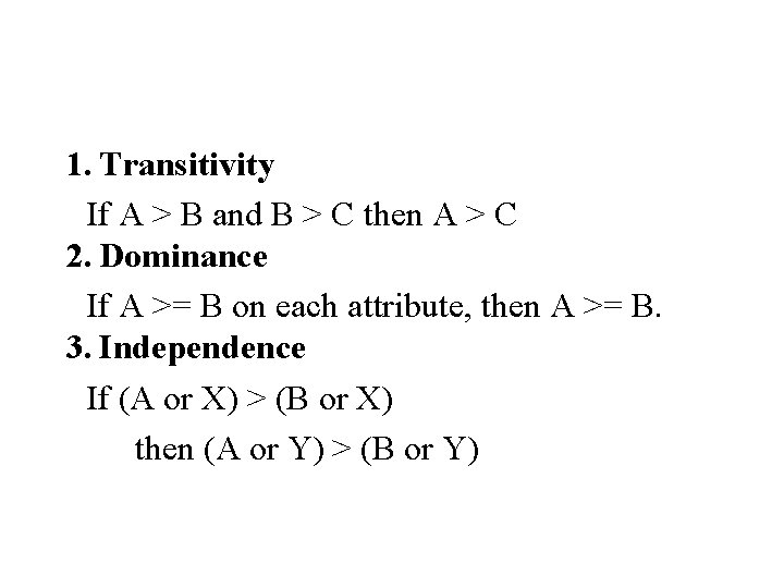
1. Transitivity If A > B and B > C then A > C 2. Dominance If A >= B on each attribute, then A >= B. 3. Independence If (A or X) > (B or X) then (A or Y) > (B or Y)

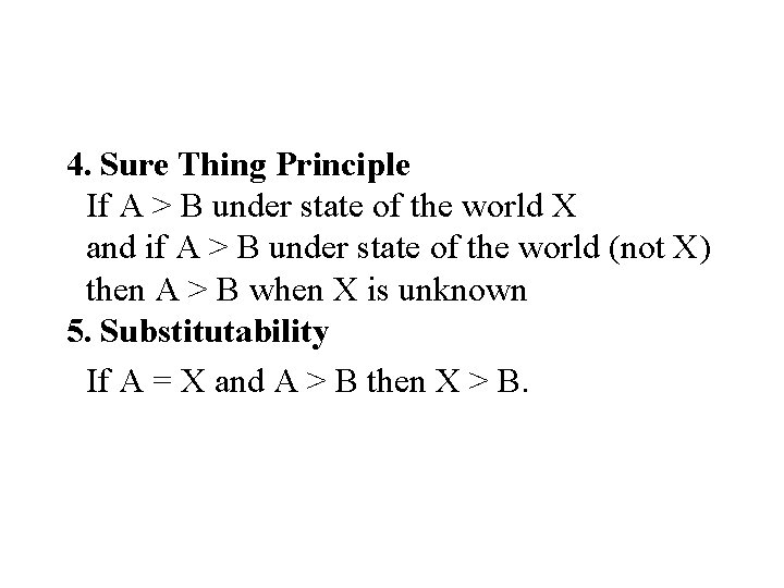
4. Sure Thing Principle If A > B under state of the world X and if A > B under state of the world (not X) then A > B when X is unknown 5. Substitutability If A = X and A > B then X > B.

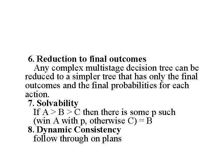
6. Reduction to final outcomes Any complex multistage decision tree can be reduced to a simpler tree that has only the final outcomes and the final probabilities for each action. 7. Solvability If A > B > C then there is some p such (win A with p, otherwise C) = B 8. Dynamic Consistency follow through on plans

How does EU follow from these axioms? Assume A > B > C > D > E are certain payoffs (e. g life years) Set u(A) = 1, u(E) = 0

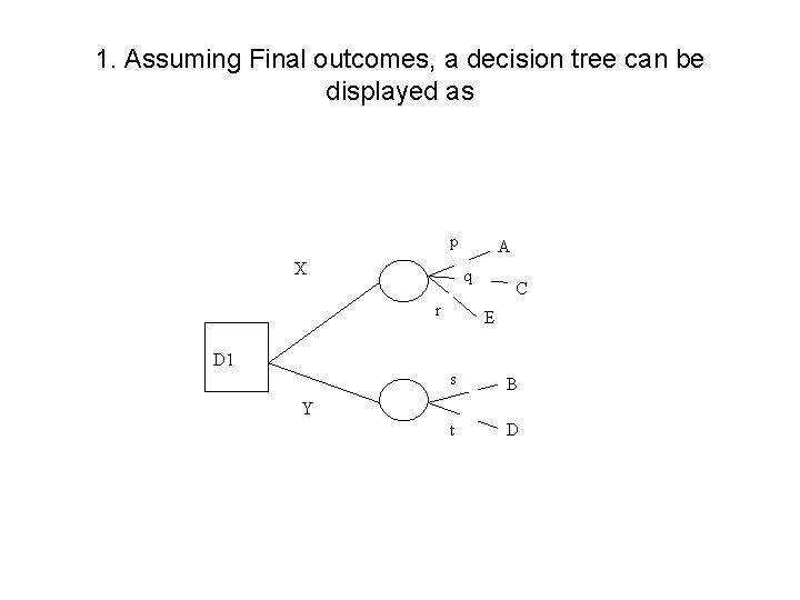
1. Assuming Final outcomes, a decision tree can be displayed as p X q r D 1 A C E s B t D Y

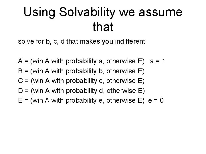
Using Solvability we assume that solve for b, c, d that makes you indifferent A = (win A with probability a, otherwise E) a = 1 B = (win A with probability b, otherwise E) C = (win A with probability c, otherwise E) D = (win A with probability d, otherwise E) E = (win A with probability e, otherwise E) e = 0

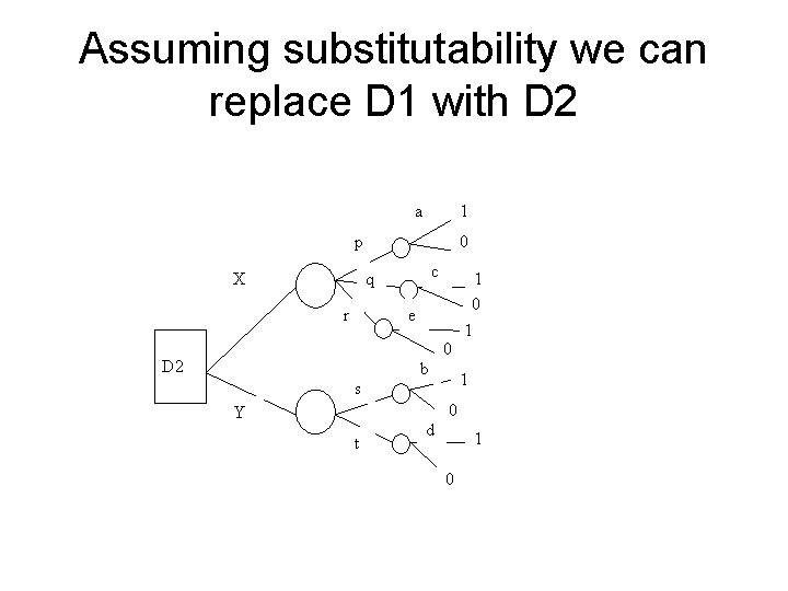
Assuming substitutability we can replace D 1 with D 2 a 1 p 0 c q X 1 0 e r D 2 b s Y t d 0 a 0 1 1 a 1 0

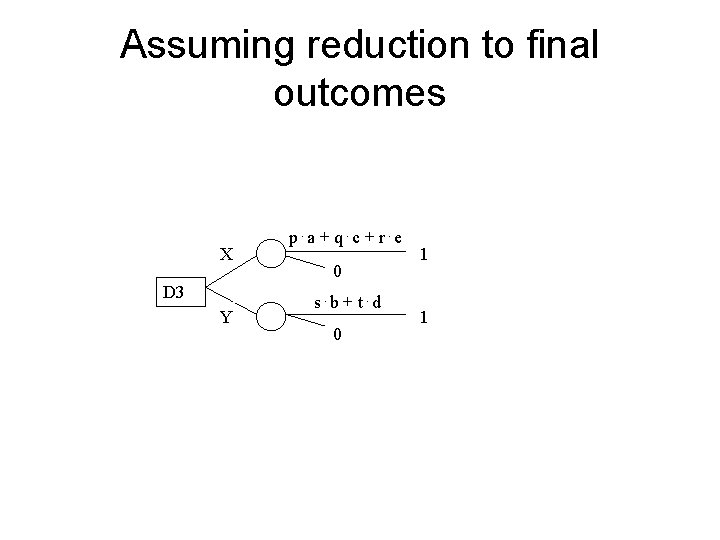
Assuming reduction to final outcomes X D 3 Y p⋅a + q⋅c + r⋅e 0 s⋅b + t⋅d 0 1 1

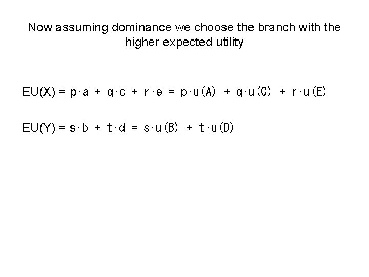
Now assuming dominance we choose the branch with the higher expected utility EU(X) = p⋅a + q⋅c + r⋅e = p⋅u(A) + q⋅u(C) + r⋅u(E) EU(Y) = s⋅b + t⋅d = s⋅u(B) + t⋅u(D)

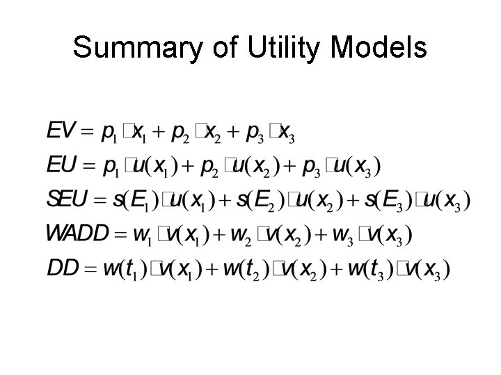
Summary of Utility Models