The Stochastic Capacity Constraint CSC 444 F05 Lecture

The Stochastic Capacity Constraint CSC 444 F'05 Lecture 5 1

MIDTERM NEW DATE AND TIME AND PLACE Tuesday, November 1 8 pm to 9 pm Woodsworth College WW 111 CSC 444 F'05 Lecture 5 2

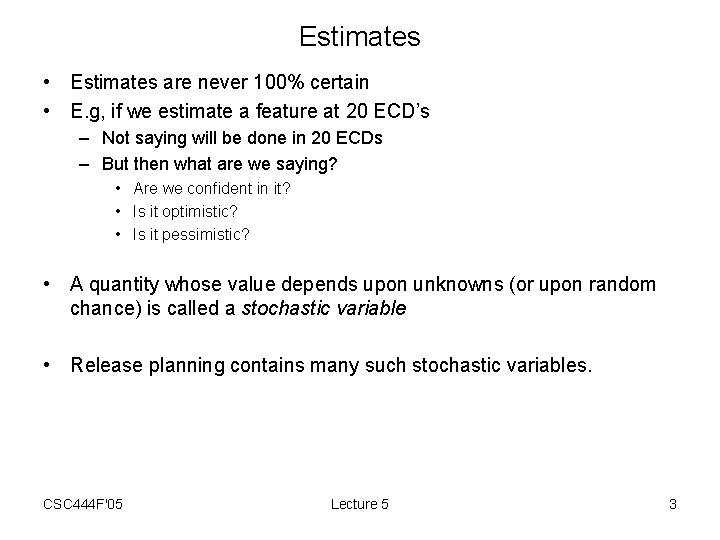
Estimates • Estimates are never 100% certain • E. g, if we estimate a feature at 20 ECD’s – Not saying will be done in 20 ECDs – But then what are we saying? • Are we confident in it? • Is it optimistic? • Is it pessimistic? • A quantity whose value depends upon unknowns (or upon random chance) is called a stochastic variable • Release planning contains many such stochastic variables. CSC 444 F'05 Lecture 5 3

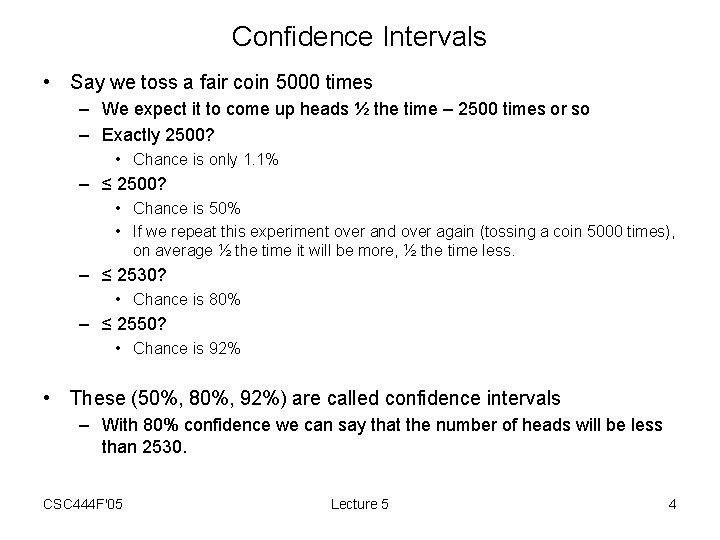
Confidence Intervals • Say we toss a fair coin 5000 times – We expect it to come up heads ½ the time – 2500 times or so – Exactly 2500? • Chance is only 1. 1% – ≤ 2500? • Chance is 50% • If we repeat this experiment over and over again (tossing a coin 5000 times), on average ½ the time it will be more, ½ the time less. – ≤ 2530? • Chance is 80% – ≤ 2550? • Chance is 92% • These (50%, 80%, 92%) are called confidence intervals – With 80% confidence we can say that the number of heads will be less than 2530. CSC 444 F'05 Lecture 5 4

Stochastic Variables • Consider the work factor of a coder, w. – When estimating in advance, w is a stochastic variable. – Stochastic variables are described by statistical distributions – A statistical distribution will tell you: • For any range of w • The probability of w being within that range – Can be described completely with a probability density function. • X-axis: all possible values of the stochastic variable • Y-axis: numbers >= 0 • The probability that the stochastic variables lies between two values a and b is given by the area under the p. d. f. between a and b. CSC 444 F'05 Lecture 5 5

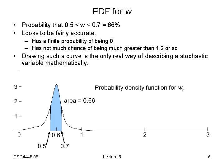
PDF for w • Probability that 0. 5 < w < 0. 7 = 66% • Looks to be fairly accurate. – Has a finite probability of being 0 – Has not much chance of being much greater than 1. 2 or so • Drawing such a curve is the only real way of describing a stochastic variable mathematically. CSC 444 F'05 Lecture 5 6

Parameterized Distributions • “So, Bill, here’s a piece of paper, could you please draw me a p. d. f. for your work factor? ” – Nobody knows the distribution to this level of accuracy – Very hard to work with mathematically • Usual method is to make an assumption about the overall shape of the curve, choosing from a few set shapes that are easy to work with mathematically. • Then ask Bill for a few parameters that we can use to fit the curve. • Because we are not so sure on our estimates anyways, the relative inaccuracy of choosing from one of a set of mathematically tractable p. d. f. ’s is small compared to the other estimation errors. CSC 444 F'05 Lecture 5 7

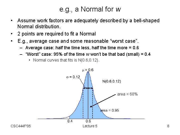
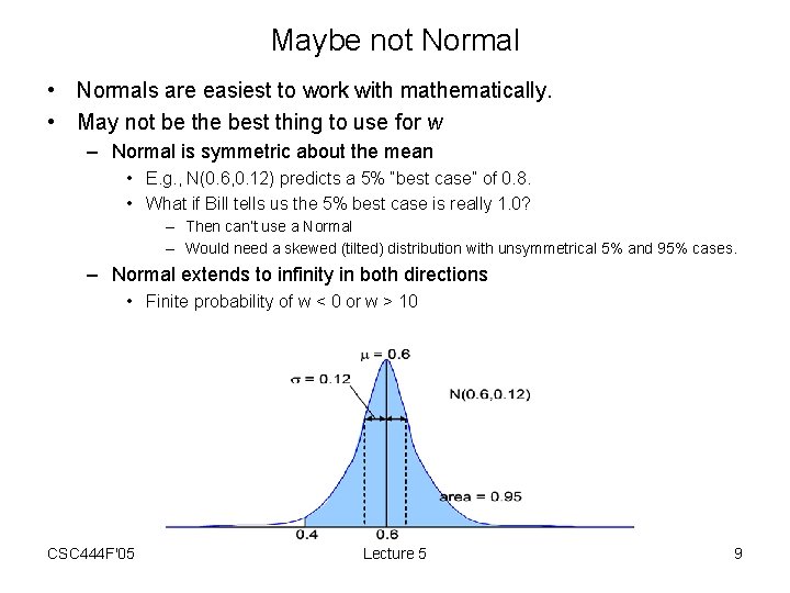
e. g. , a Normal for w • Assume work factors are adequately described by a bell-shaped Normal distribution. • 2 points are required to fit a Normal • E. g. , average case and some reasonable “worst case”. – Average case: half the time less, half the time more = 0. 6 – “Worst” case: 95% of the time w won’t be that bad (small) = 0. 4 • Normal curves that fits is N(0. 6, 0. 12). area = 68% CSC 444 F'05 Lecture 5 8

Maybe not Normal • Normals are easiest to work with mathematically. • May not be the best thing to use for w – Normal is symmetric about the mean • E. g. , N(0. 6, 0. 12) predicts a 5% “best case” of 0. 8. • What if Bill tells us the 5% best case is really 1. 0? – Then can’t use a Normal – Would need a skewed (tilted) distribution with unsymmetrical 5% and 95% cases. – Normal extends to infinity in both directions • Finite probability of w < 0 or w > 10 CSC 444 F'05 Lecture 5 9

Estimates • Most define our quantities very precisely • E. g. , for a feature estimate of 1 week – Post-Facto • What are the units? • 40 hours? Longer? Shorter? Dedicated? Disrupted? One person or two? . . . • Dealt with this last lecture in great detail – Stochastic • • 1 week best case? 1 week worst case? 1 week average case? Need a p. d. f • Depending upon these concerns, my “ 1 week” maybe somebody else’s 4 weeks. – Very significant issue in practice CSC 444 F'05 Lecture 5 10

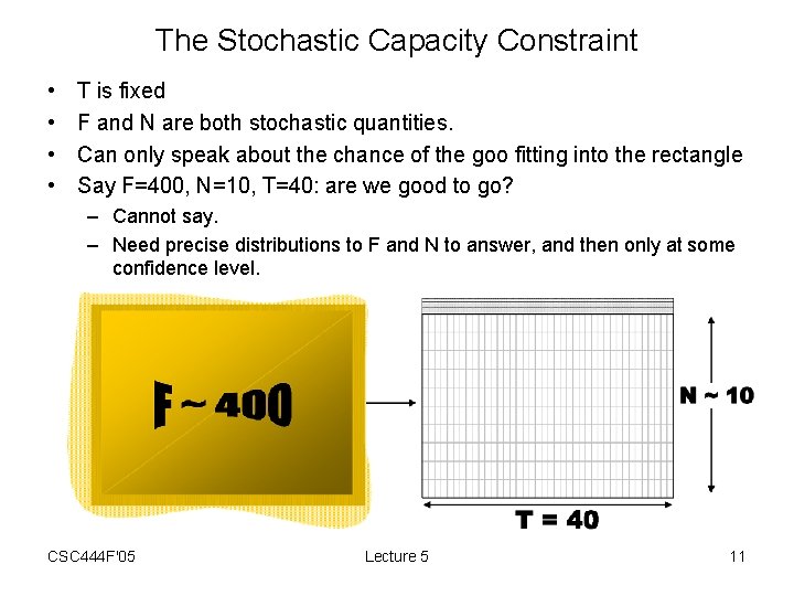
The Stochastic Capacity Constraint • • T is fixed F and N are both stochastic quantities. Can only speak about the chance of the goo fitting into the rectangle Say F=400, N=10, T=40: are we good to go? – Cannot say. – Need precise distributions to F and N to answer, and then only at some confidence level. CSC 444 F'05 Lecture 5 11

Summing Distributions • • F and N are sums and products over many contributing stochastic variables. E. g. – F = f 1 + f 2 – If f 1 and f 2 have associated statistical distributions, what is the statistical distribution of F? – In general, no answer. – Special case: f 1 and f 2 are both Normal • Then F will be Normal as well. • Mean of F will be the sums of the means of f 1 and f 2 • Standard deviation of F will be the square root of the sums of the squares of the standard deviations of f 1 and f 2. – How about f 1 * f 2? • Figet about it! Huge formula, result is not a Normal distribution – One needs statistical simulation software tools to do arithmetic on stochastic variables. CSC 444 F'05 Lecture 5 12

Law of Large Numbers • If we sum lots and lots of stochastic variables, the sum will approach a Normal distribution. • Therefore something like F is going to be pretty close to Normal. – E. g. , 400 features summed • N will also be, but a bit less so – E. g. , 10 w’s summed CSC 444 F'05 Lecture 5 13

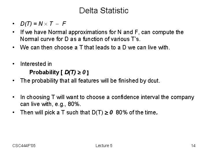
Delta Statistic • D(T) = N T F • If we have Normal approximations for N and F, can compute the Normal curve for D as a function of various T’s. • We can then choose a T that leads to a D we can live with. • Interested in Probability [ D(T) 0 ] • The probability that all features will be finished by dcut. • In choosing T will want to choose a confidence interval the company can live with, e. g. , 80%. • Then will pick a T such that D(T) 0 80% of the time. CSC 444 F'05 Lecture 5 14

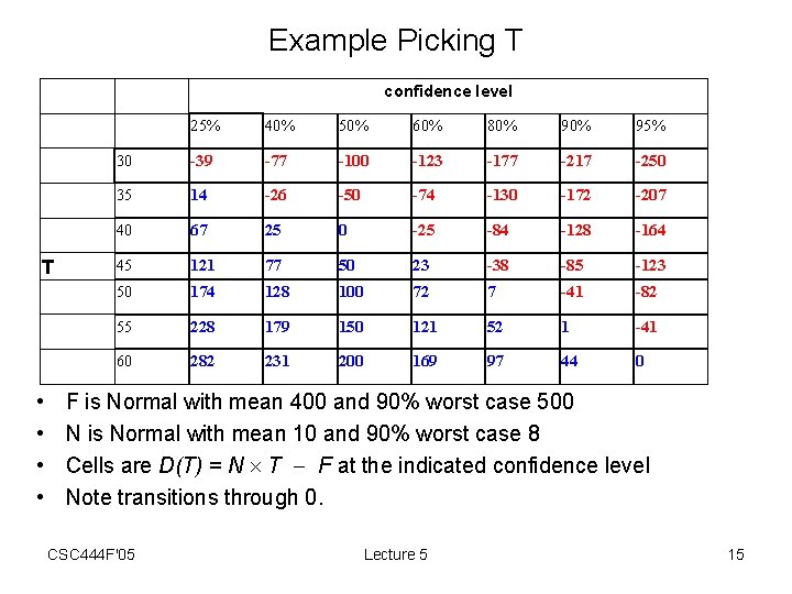
Example Picking T confidence level T • • 25% 40% 50% 60% 80% 95% 30 -39 -77 -100 -123 -177 -217 -250 35 14 -26 -50 -74 -130 -172 -207 40 67 25 0 -25 -84 -128 -164 45 121 77 50 23 -38 -85 -123 50 174 128 100 72 7 -41 -82 55 228 179 150 121 52 1 -41 60 282 231 200 169 97 44 0 F is Normal with mean 400 and 90% worst case 500 N is Normal with mean 10 and 90% worst case 8 Cells are D(T) = N T F at the indicated confidence level Note transitions through 0. CSC 444 F'05 Lecture 5 15

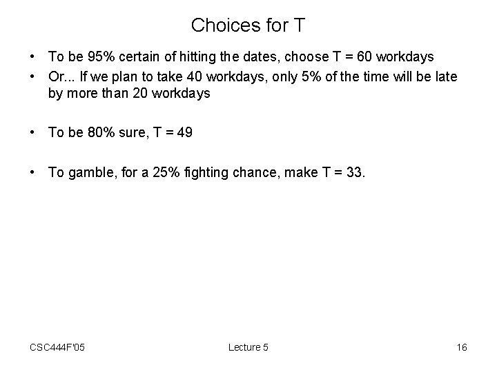
Choices for T • To be 95% certain of hitting the dates, choose T = 60 workdays • Or. . . If we plan to take 40 workdays, only 5% of the time will be late by more than 20 workdays • To be 80% sure, T = 49 • To gamble, for a 25% fighting chance, make T = 33. CSC 444 F'05 Lecture 5 16

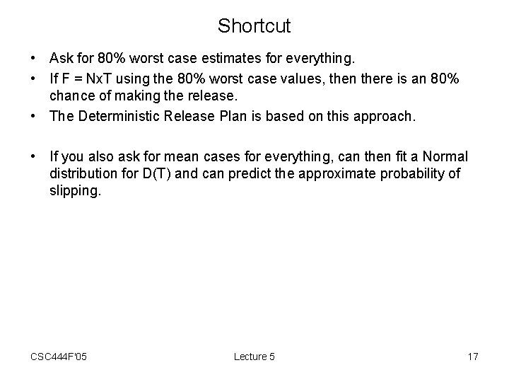
Shortcut • Ask for 80% worst case estimates for everything. • If F = Nx. T using the 80% worst case values, then there is an 80% chance of making the release. • The Deterministic Release Plan is based on this approach. • If you also ask for mean cases for everything, can then fit a Normal distribution for D(T) and can predict the approximate probability of slipping. CSC 444 F'05 Lecture 5 17

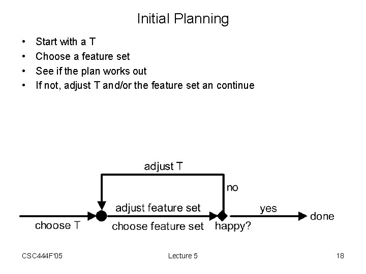
Initial Planning • • Start with a T Choose a feature set See if the plan works out If not, adjust T and/or the feature set an continue CSC 444 F'05 Lecture 5 18

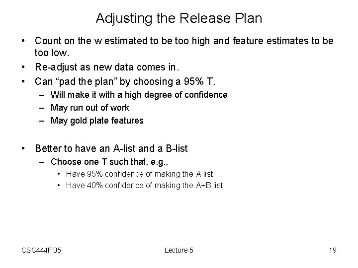
Adjusting the Release Plan • Count on the w estimated to be too high and feature estimates to be too low. • Re-adjust as new data comes in. • Can “pad the plan” by choosing a 95% T. – Will make it with a high degree of confidence – May run out of work – May gold plate features • Better to have an A-list and a B-list – Choose one T such that, e. g. , • Have 95% confidence of making the A list • Have 40% confidence of making the A+B list. CSC 444 F'05 Lecture 5 19

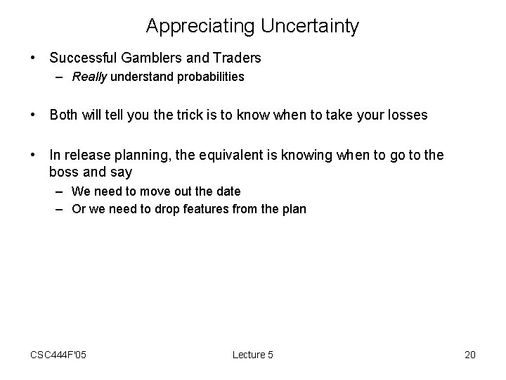
Appreciating Uncertainty • Successful Gamblers and Traders – Really understand probabilities • Both will tell you the trick is to know when to take your losses • In release planning, the equivalent is knowing when to go to the boss and say – We need to move out the date – Or we need to drop features from the plan CSC 444 F'05 Lecture 5 20

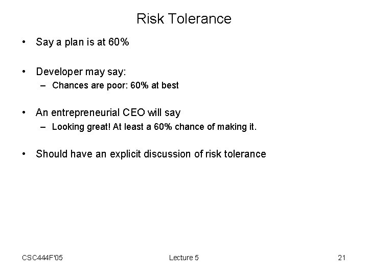
Risk Tolerance • Say a plan is at 60% • Developer may say: – Chances are poor: 60% at best • An entrepreneurial CEO will say – Looking great! At least a 60% chance of making it. • Should have an explicit discussion of risk tolerance CSC 444 F'05 Lecture 5 21

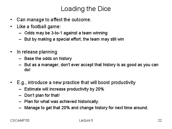
Loading the Dice • Can manage to affect the outcome. • Like a football game: – Odds may be 3 -to-1 against a team winning – But by making a special effort, the team may still win • In release planning – Base the odds on history – But as a manager, don’t ever accept that history is as good as you can do! • E. g. , introduce a new practice that will boost productivity – – Estimate will increase productivity by 20% Don’t plan for that! Plan for what was achieved historically. Manage to get that 20% and change history for next time around. CSC 444 F'05 Lecture 5 22

Example Stochastic Release Plan • Sample Stochastic Release Plan CSC 444 F'05 Lecture 5 23