The Canadian Lynx vs the Snowshoe Hare The

- Slides: 8

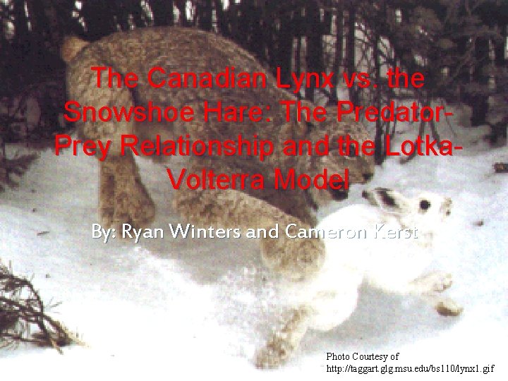
The Canadian Lynx vs. the Snowshoe Hare: The Predator. Prey Relationship and the Lotka. Volterra Model By: Ryan Winters and Cameron Kerst Photo Courtesy of http: //taggart. glg. msu. edu/bs 110/lynx 1. gif

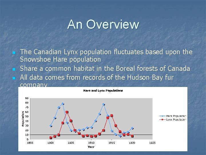
An Overview n n n The Canadian Lynx population fluctuates based upon the Snowshoe Hare population Share a common habitat in the Boreal forests of Canada All data comes from records of the Hudson Bay fur company

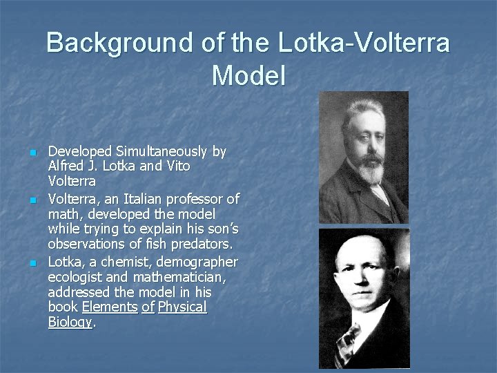
Background of the Lotka-Volterra Model n n n Developed Simultaneously by Alfred J. Lotka and Vito Volterra, an Italian professor of math, developed the model while trying to explain his son’s observations of fish predators. Lotka, a chemist, demographer ecologist and mathematician, addressed the model in his book Elements of Physical Biology.

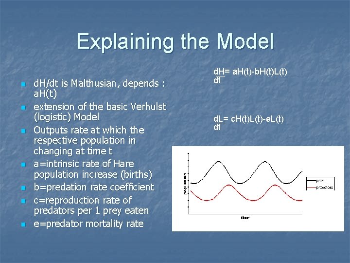
Explaining the Model n n n n d. H/dt is Malthusian, depends : a. H(t) extension of the basic Verhulst (logistic) Model Outputs rate at which the respective population in changing at time t a=intrinsic rate of Hare population increase (births) b=predation rate coefficient c=reproduction rate of predators per 1 prey eaten e=predator mortality rate d. H= a. H(t)-b. H(t)L(t) dt d. L= c. H(t)L(t)-e. L(t) dt

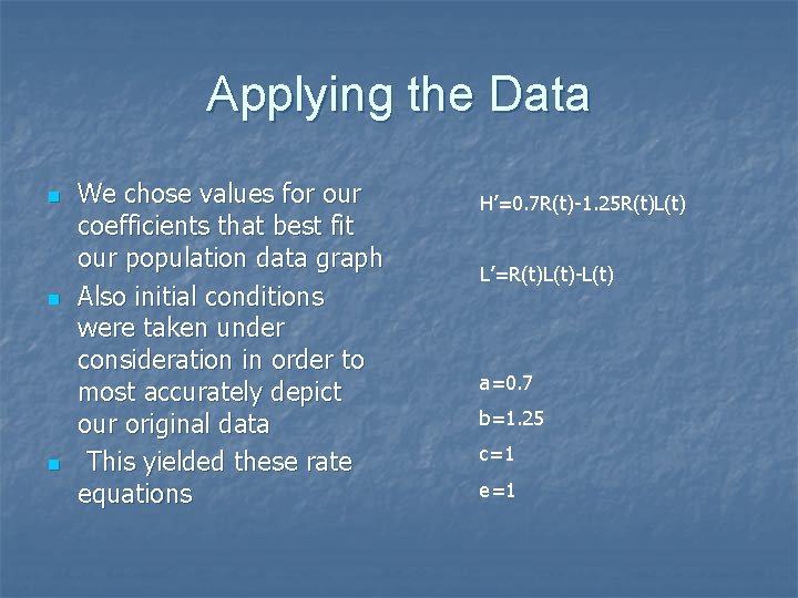
Applying the Data n n n We chose values for our coefficients that best fit our population data graph Also initial conditions were taken under consideration in order to most accurately depict our original data This yielded these rate equations H’=0. 7 R(t)-1. 25 R(t)L(t) L’=R(t)L(t)-L(t) a=0. 7 b=1. 25 c=1 e=1

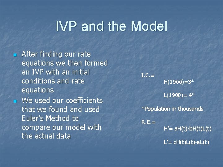
IVP and the Model n n After finding our rate equations we then formed an IVP with an initial conditions and rate equations We used our coefficients that we found and used Euler’s Method to compare our model with the actual data I. C. = H(1900)=3* L(1900)=. 4* *Population in thousands R. E. = H’= a. H(t)-b. H(t)L(t) L’= c. H(t)L(t)-e. L(t)

Works Consulted n n n n Works Consulted: Lotka, Alfred J. Elements of Physical Biology. Mahaffy, Joseph M. “Lotka-Volterra Models. ” San Diego State University: 2000. http: //wwwrohan. sdsu. edu/~jmahaffy/courses/f 00/math 122/lectures/qual_de 2/qualde 2. ht ml Mc. Kelvey, Steve. “Lotka-Volterra Two Species Model. ” <http: //www. stolaf. edu/people/mckelvey/envision. dir/lotka-volt. html > Sharov, Alexei. “Lotka-Volterra Model. ” 01/12/1996. < http: //www. gypsymoth. ento. vt. edu/~sharov/Pop. Ecol/lec 10/lotka. html > “Vito Voltera. ” School of Mathematics and Statistics, University of St. Andrews, Scotland. December 1996. < http: //www-groups. dcs. stand. ac. uk/~history/Mathematicians/Volterra. html > “Alfred J. Lotka. ” Wikipedia. <http: //www. stolaf. edu/people/mckelvey/envision. dir/lotka-volt. html > 12/01/2005

The End Thank You!!!