SSACgnp TD 883 DKM 1 4 What are

SSACgnp. TD 883. DKM 1. 4 What are the Winds Blowing into Mammoth Cave? The concentration of surface air pollutants is of growing concern at Mammoth Cave National Park, but what volume of pollutants is making it into the cave? Core Quantitative Issue Modeling and estimation USGS Supporting Quantitative Literacy Topic Basic arithmetic Proportions Graphical representation of data Core Geoscience Subject Air quality; Cave management Dorien K. Mc. Gee 1, Bobby Carson 2, and Jonathan Jernigan 3; 1 Department of Geology, University of South Florida, Tampa, FL 33620; 2 Mammoth Cave National Park, Mammoth Cave, KY 42259; 3 Cumberland Piedmont Network, Mammoth Cave National Park, Mammoth Cave, KY 42259 © 2010 University of South Florida Libraries. All rights reserved. This material is based upon work supported by the National Science Foundation under Grant Number NSF DUE-0836566. Any opinions, findings, and conclusions or recommendations expressed in this material are those of the author(s) and do not necessarily reflect the views of the National Science Foundation. 1

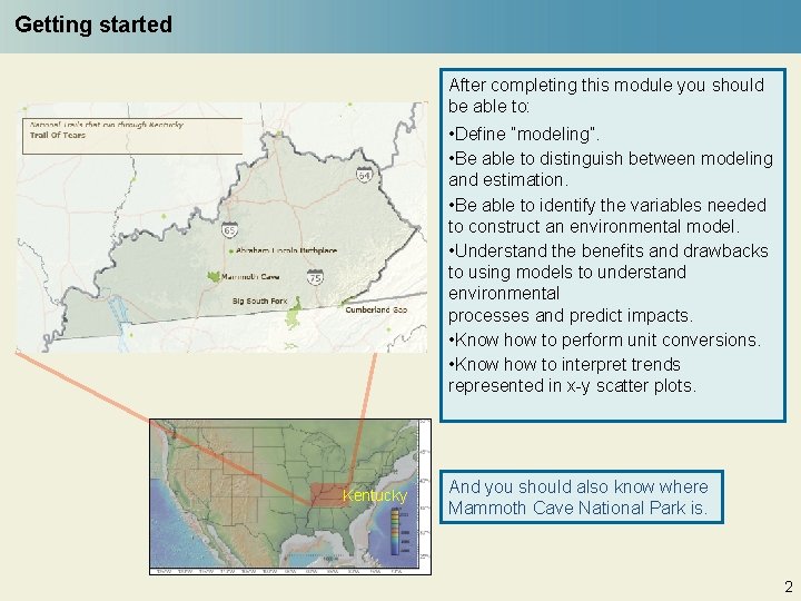
Getting started After completing this module you should be able to: • Define “modeling”. • Be able to distinguish between modeling and estimation. • Be able to identify the variables needed to construct an environmental model. • Understand the benefits and drawbacks to using models to understand environmental processes and predict impacts. • Know how to perform unit conversions. • Know how to interpret trends represented in x-y scatter plots. Kentucky And you should also know where Mammoth Cave National Park is. 2

The setting – Mammoth Cave National Park is the most extensive known cave system in the world and was recognized as a World Heritage Site in 1981 and as an International Biosphere Reserve in 1990. The cave has been forming in stages over the last 10 million years, contains almost every known type of cave formation, and is the most biodiverse cave system known in the world. The relative stability of cave environment helps preserve both its features and its organisms; however, this makes them more sensitive to perturbations such as changes in the flow and/or chemistry of the air and water. These perturbations are often triggered by anthropogenic activities at the surface. Air quality at the surface of Mammoth Cave is of utmost concern due to pollutants drifting south from coal processing and other industrial activities in the Ohio River Valley. Sinkhole plain Soda straw Green River Frozen Niagara 3

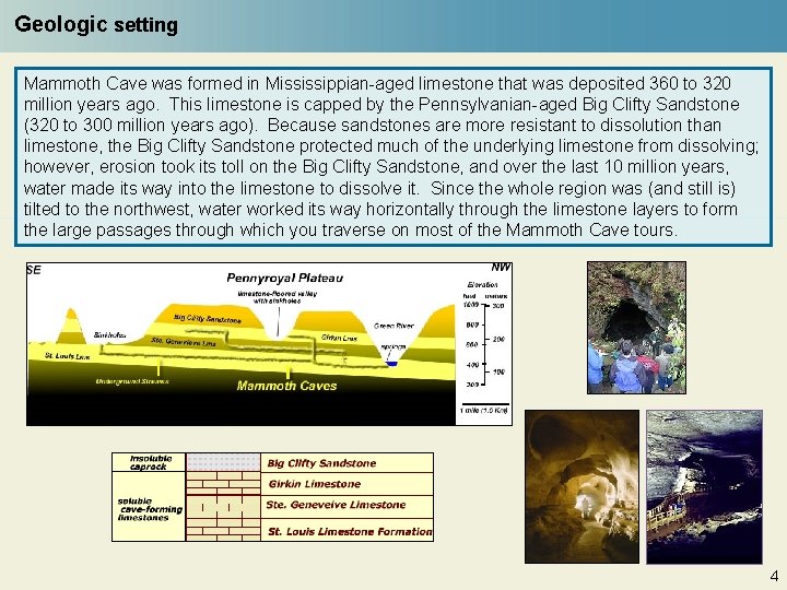
Geologic setting Mammoth Cave was formed in Mississippian-aged limestone that was deposited 360 to 320 million years ago. This limestone is capped by the Pennsylvanian-aged Big Clifty Sandstone (320 to 300 million years ago). Because sandstones are more resistant to dissolution than limestone, the Big Clifty Sandstone protected much of the underlying limestone from dissolving; however, erosion took its toll on the Big Clifty Sandstone, and over the last 10 million years, water made its way into the limestone to dissolve it. Since the whole region was (and still is) tilted to the northwest, water worked its way horizontally through the limestone layers to form the large passages through which you traverse on most of the Mammoth Cave tours. 4

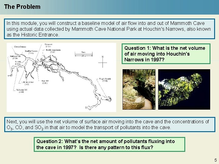
The Problem In this module, you will construct a baseline model of air flow into and out of Mammoth Cave using actual data collected by Mammoth Cave National Park at Houchin's Narrows, also known as the Historic Entrance. Question 1: What is the net volume of air moving into Houchin's Narrows in 1997? Next, you will use the net volume of surface air moving into the cave and the concentrations of O 3, CO, and SO 2 in that air to model the transport of pollutants into the cave. Question 2: What’s the net amount of pollutants fluxing into the cave in 1997? Is there any pattern to this flux? 5

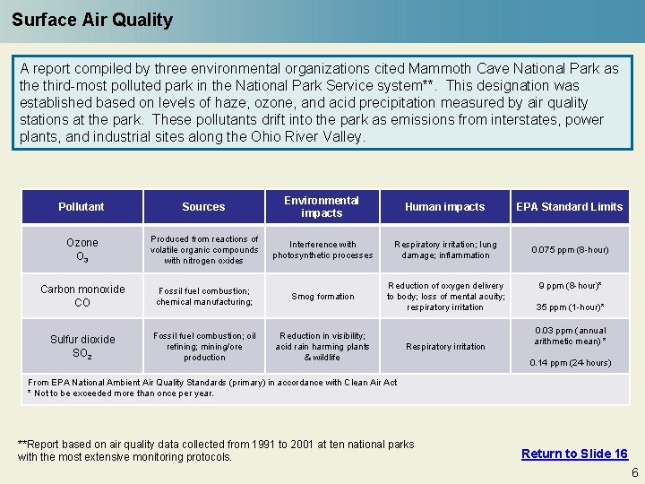
Surface Air Quality A report compiled by three environmental organizations cited Mammoth Cave National Park as the third-most polluted park in the National Park Service system**. This designation was established based on levels of haze, ozone, and acid precipitation measured by air quality stations at the park. These pollutants drift into the park as emissions from interstates, power plants, and industrial sites along the Ohio River Valley. Pollutant Sources Environmental impacts Human impacts EPA Standard Limits Ozone O 3 Produced from reactions of volatile organic compounds with nitrogen oxides Interference with photosynthetic processes Respiratory irritation; lung damage; inflammation 0. 075 ppm (8 -hour) Carbon monoxide CO Fossil fuel combustion; chemical manufacturing; Smog formation Reduction of oxygen delivery to body; loss of mental acuity; respiratory irritation Sulfur dioxide SO 2 Fossil fuel combustion; oil refining; mining/ore production Reduction in visibility; acid rain harming plants & wildlife Respiratory irritation 9 ppm (8 -hour)* 35 ppm (1 -hour)* 0. 03 ppm (annual arithmetic mean) * 0. 14 ppm (24 -hours) From EPA National Ambient Air Quality Standards (primary) in accordance with Clean Air Act * Not to be exceeded more than once per year. **Report based on air quality data collected from 1991 to 2001 at ten national parks with the most extensive monitoring protocols. Return to Slide 16 6

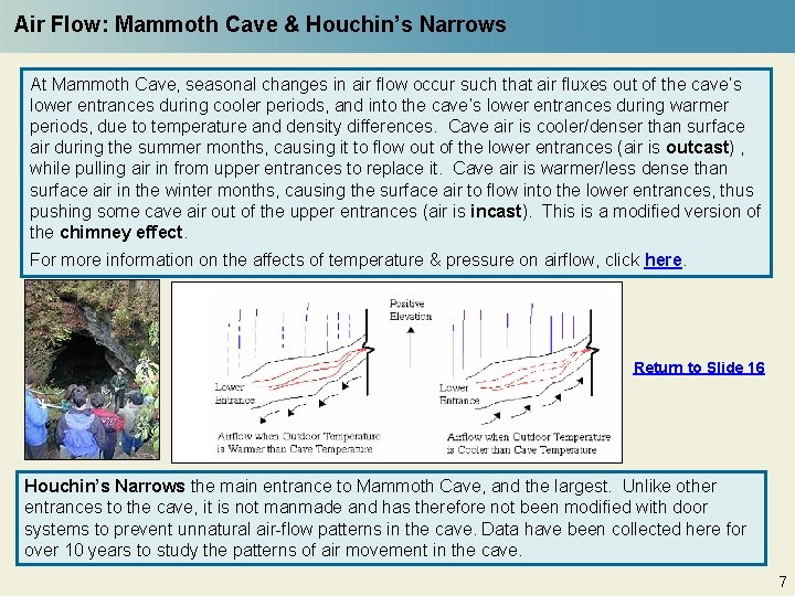
Air Flow: Mammoth Cave & Houchin’s Narrows At Mammoth Cave, seasonal changes in air flow occur such that air fluxes out of the cave’s lower entrances during cooler periods, and into the cave’s lower entrances during warmer periods, due to temperature and density differences. Cave air is cooler/denser than surface air during the summer months, causing it to flow out of the lower entrances (air is outcast) , while pulling air in from upper entrances to replace it. Cave air is warmer/less dense than surface air in the winter months, causing the surface air to flow into the lower entrances, thus pushing some cave air out of the upper entrances (air is incast). This is a modified version of the chimney effect. For more information on the affects of temperature & pressure on airflow, click here. Return to Slide 16 Houchin’s Narrows the main entrance to Mammoth Cave, and the largest. Unlike other entrances to the cave, it is not manmade and has therefore not been modified with door systems to prevent unnatural air-flow patterns in the cave. Data have been collected here for over 10 years to study the patterns of air movement in the cave. 7

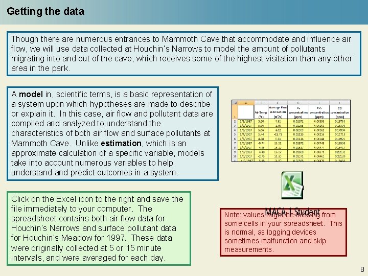
Getting the data Though there are numerous entrances to Mammoth Cave that accommodate and influence air flow, we will use data collected at Houchin’s Narrows to model the amount of pollutants migrating into and out of the cave, which receives some of the highest visitation than any other area in the park. A model in, scientific terms, is a basic representation of a system upon which hypotheses are made to describe or explain it. In this case, air flow and pollutant data are compiled analyzed to understand the characteristics of both air flow and surface pollutants at Mammoth Cave. Unlike estimation, which is an approximate calculation of a specific variable, models take into account numerous variables to help understand predict outcomes in a system. Click on the Excel icon to the right and save the file immediately to your computer. The spreadsheet contains both air flow data for Houchin’s Narrows and surface pollutant data for Houchin’s Meadow for 1997. These data were originally collected at 5 or 15 minute intervals, and were averaged for each day. Note: values might be missing from some cells in your spreadsheet. This is normal, as logging devices sometimes malfunction and skip measurements. 8

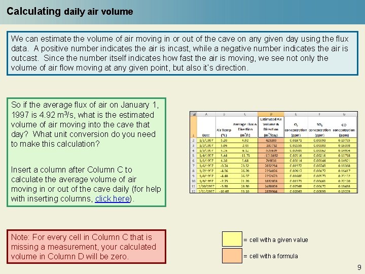
Calculating daily air volume We can estimate the volume of air moving in or out of the cave on any given day using the flux data. A positive number indicates the air is incast, while a negative number indicates the air is outcast. Since the number itself indicates how fast the air is moving, we see not only the volume of air flow moving at any given point, but also it’s direction. So if the average flux of air on January 1, 1997 is 4. 92 m 3/s, what is the estimated volume of air moving into the cave that day? What unit conversion do you need to make this calculation? Insert a column after Column C to calculate the average volume of air moving in or out of the cave daily (for help with inserting columns, click here). Note: For every cell in Column C that is missing a measurement, your calculated volume in Column D will be zero. = cell with a given value = cell with a formula 9

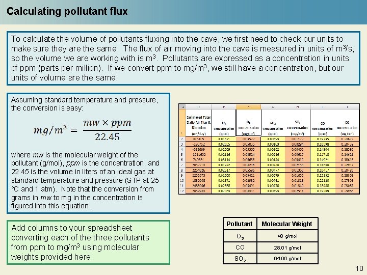
Calculating pollutant flux To calculate the volume of pollutants fluxing into the cave, we first need to check our units to make sure they are the same. The flux of air moving into the cave is measured in units of m 3/s, so the volume we are working with is m 3. Pollutants are expressed as a concentration in units of ppm (parts per million). If we convert ppm to mg/m 3, we still have a concentration, but our units of volume are the same. Assuming standard temperature and pressure, the conversion is easy: where mw is the molecular weight of the pollutant (g/mol), ppm is the concentration, and 22. 45 is the volume in liters of an ideal gas at standard temperature and pressure (STP at 25 °C and 1 atm). Note that the conversion from grams in mw to mg in the concentration is figured into this equation. Add columns to your spreadsheet converting each of the three pollutants from ppm to mg/m 3 using molecular weights provided here. Pollutant Molecular Weight O 3 48 g/mol CO 28. 01 g/mol SO 2 64. 06 g/mol 10

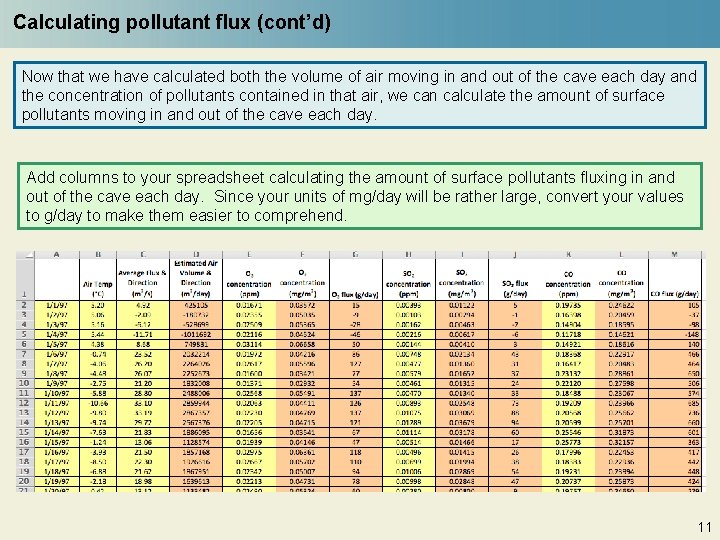
Calculating pollutant flux (cont’d) Now that we have calculated both the volume of air moving in and out of the cave each day and the concentration of pollutants contained in that air, we can calculate the amount of surface pollutants moving in and out of the cave each day. Add columns to your spreadsheet calculating the amount of surface pollutants fluxing in and out of the cave each day. Since your units of mg/day will be rather large, convert your values to g/day to make them easier to comprehend. 11

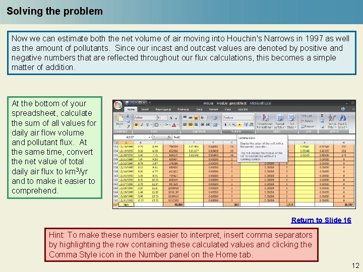
Solving the problem Now we can estimate both the net volume of air moving into Houchin's Narrows in 1997 as well as the amount of pollutants. Since our incast and outcast values are denoted by positive and negative numbers that are reflected throughout our flux calculations, this becomes a simple matter of addition. At the bottom of your spreadsheet, calculate the sum of all values for daily air flow volume and pollutant flux. At the same time, convert the net value of total daily air flux to km 3/yr and to make it easier to comprehend. Return to Slide 16 Hint: To make these numbers easier to interpret, insert comma separators by highlighting the row containing these calculated values and clicking the Comma Style icon in the Number panel on the Home tab. 12

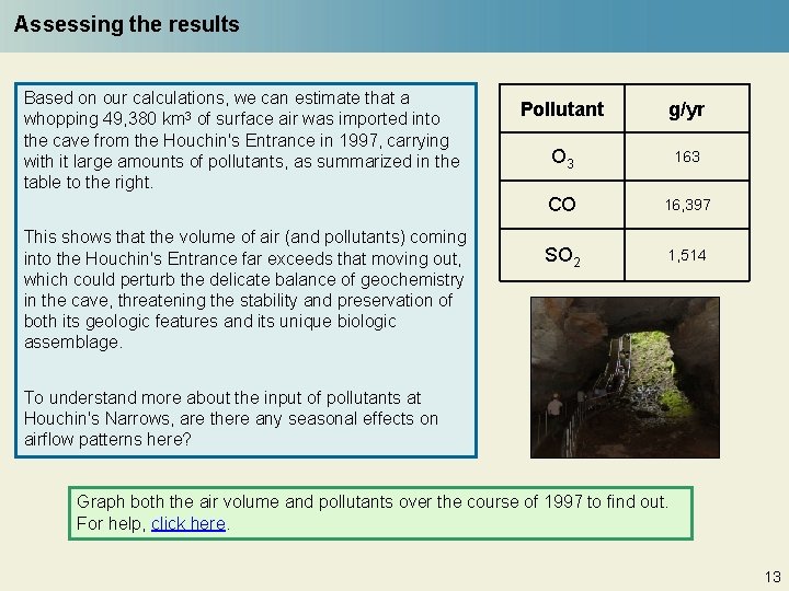
Assessing the results Based on our calculations, we can estimate that a whopping 49, 380 km 3 of surface air was imported into the cave from the Houchin's Entrance in 1997, carrying with it large amounts of pollutants, as summarized in the table to the right. This shows that the volume of air (and pollutants) coming into the Houchin's Entrance far exceeds that moving out, which could perturb the delicate balance of geochemistry in the cave, threatening the stability and preservation of both its geologic features and its unique biologic assemblage. Pollutant g/yr O 3 163 CO 16, 397 SO 2 1, 514 To understand more about the input of pollutants at Houchin's Narrows, are there any seasonal effects on airflow patterns here? Graph both the air volume and pollutants over the course of 1997 to find out. For help, click here. 13

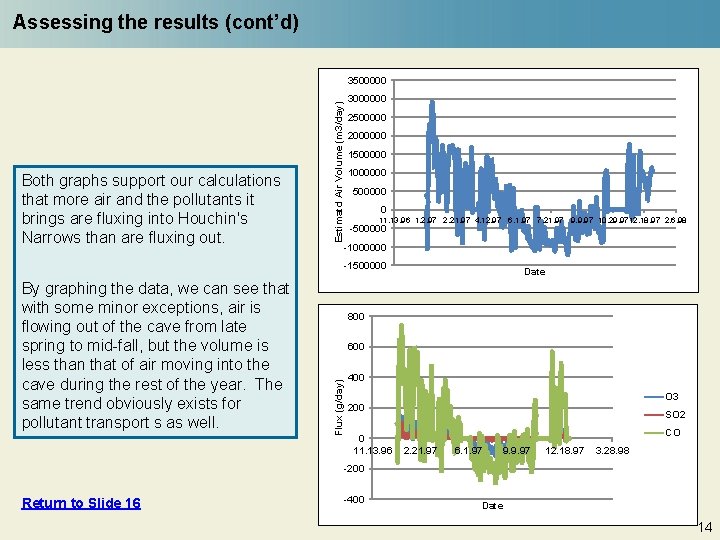
Assessing the results (cont’d) Both graphs support our calculations that more air and the pollutants it brings are fluxing into Houchin's Narrows than are fluxing out. Estimatd Air Volume (m 3/day) 3500000 3000000 2500000 2000000 1500000 1000000 500000 0 11. 13. 96 1. 2. 97 2. 21. 97 4. 12. 97 6. 1. 97 7. 21. 97 9. 9. 97 10. 29. 9712. 18. 97 2. 6. 98 -500000 -1000000 -1500000 800 600 Flux (g/day) By graphing the data, we can see that with some minor exceptions, air is flowing out of the cave from late spring to mid-fall, but the volume is less than that of air moving into the cave during the rest of the year. The same trend obviously exists for pollutant transport s as well. Date 400 O 3 200 0 11. 13. 96 SO 2 CO 2. 21. 97 6. 1. 97 9. 9. 97 12. 18. 97 3. 28. 98 -200 Return to Slide 16 -400 Date 14

Wrap-up: assumptions in modeling During the course of these calculations, you should have noticed we’re making some very important assumptions: 1. We are assuming standard temperature and pressure when converting the concentration of pollutants from ppm to mg/m 3. 2. We are assuming that missing data from malfunctioning data loggers would not contradict our results. 3. Trends seen at Houchin's Narrows in 1997 are indicative of long-term trends. We are also ignoring some key points: 1. What’s the net volume of surface air imported to the entire cave (accounting for the chimney effect and all entrances)? Are the patterns at Houchin's Narrows reflective of air flow patterns at other entrances? 2. What’s the residence time of surface air pollutants in the cave? Do they flux out as rapidly as they flux in or do they get trapped? Do they react with naturally-occurring elements in the cave? Making assumptions are a vital part of the modeling process because it’s often impractical, if not impossible, to account for every variable in the system you’re trying to model. Uncertainty is always a factor to consider when interpreting model results, and therefore you have to make your model as complete as your datasets will allow, knowing your model results and interpretations may change as new data becomes available. What data would you add to make this model more complete? Return to Slide 16 15

End-of-module assignment 1. Construct the spreadsheet as described in Slides 9 -12, and the x-y scatter plots as described in Slides 13 -14. 2. Answer the question at the bottom of Slide 15. 3. Create another x-y scatter plot to illustrate how air temperatures at Houchins Narrows changed over time and compare the results with your plot of air flux over time. How do air flux and air temperature co-vary? Explain in terms of the chimney effect described on Slide 7. 4. The EPA standards given on Slide 6 typically apply to 1 - and 8 -hour periods (with the exception of SO 2). The dataset you have reports pollutant concentrations as daily averages, but may still be used to estimate whether pollutants might have exceeded EPA standards in 1997. Calculate the yearly average of all three pollutants (in ppm) at the bottom of your spreadsheet. Next, use the =MAX function to identify the highest daily average for each pollutant that year. Did any averages or maximum values come close to any of the EPA standards (regardless of the time duration)? If these calculations are based on daily averages, how might you interpret how the actual measured values varied? 16

End-of-module assignment, cont’d 5. Ozone is a pollutant of concern at Mammoth Cave National Park. Its ground levels are related to vehicle and industrial emissions, but only indirectly. Using the internet as a source, describe how ozone forms from emissions. 6. Create three new x-y scatter plots to illustrate how the pollutant concentrations change over time (using ppm data). How do these three pollutants vary seasonally? If the major source of these pollutants are power plants in the Ohio River Valley, can you explain these variations? Why do you think ozone behaves differently? Hint: pollutant information on Slide 6 and your answer for Question 5 may help. 17

End-of-module assignment – intermediate/advanced In Question 3 of the End of Module assignment, we estimated whether any of the three pollutants exceeded EPA standards for 1997. Since we were using daily averages rather than raw data to assess this, we could not be certain of our results. Here we will work with raw pollutant data supplied by Mammoth Cave National Park to better address this question (it was from these data that daily averages were calculated and used earlier in this module). Since data were recorded roughly every 5 minutes, the resultant dataset has nearly 102, 000 entries for each pollutant! This is an exercise in narrowing and filtering your dataset to get the answers you need! 1. Use the MAX function to determine which, if any, of the three pollutants exceeded the concentration limits cited for 8 -hour increments (in the case of SO 2, use the 24 -hour increment). You will find that the only pollutant that exceeded the value set by an EPA standard was ozone; however, we do not know at this point whether it reached or exceeded the 0. 075 ppm threshold for 8 hours or more any given day. To determine the likelihood for this, use the COUNTIF function to identify how many data measurements are greater than or equal to 0. 075. 18

End-of-module assignment – intermediate/advanced 2. Since ozone concentrations have met or exceeded 0. 075 ppm just over 5, 900 times during the course of the dataset we stand a good chance that it has done so over an 8 -hour period. Highlight the column bearing the ozone data and select the Filter tool in the Data Panel. Click the down-arrow in the ozone column and select “Number Filters”, then “Greater Than Or Equal To” from the pop-up menu. Type in your threshhold and click OK. 3. Now that you have filtered down your data to include only points where ozone exceeded 0. 075 ppm, you may examine the data a bit closer to identify when it has held those levels for a period of 8 -hours straight. Though we could examine the whole dataset, for this exercise we will only do it for the first two weeks of August, One of the higher months. Filter the date to include only values for August, then further filter to include only the first 14 days. 4. There are 24 days in the month of August with high ozone concentrations. Scroll through these data and list which dates ozone met and/or exceeded the 8 -hour EPA standard. Be sure you have full hours (i. e. , if your data start at 14: 30, you should have values for every 5 minutes until at least 22: 30). Did any other days come close? Record your results and hand in your spreadsheets. 19

References Slide 5 – images from Dr. Lindley Hanson, Salem State College Department of Geological Sciences Slide 6 – Sources: USA Today, Appalachian Voice, Slide 7 – image by Jonathan Jernigan: “Mathematical Modeling of Convective Heat Transfer in Mammoth Cave” (MS Thesis, Western Kentucky University, 1997). Slide 22 – upper image from Technical. Engineering. org; bottom left image from Charles Sturt University; bottom right image from Meteorological Monsters laboratory exercise (Science Education Resource Center). Slide 23 – map from NPS 20

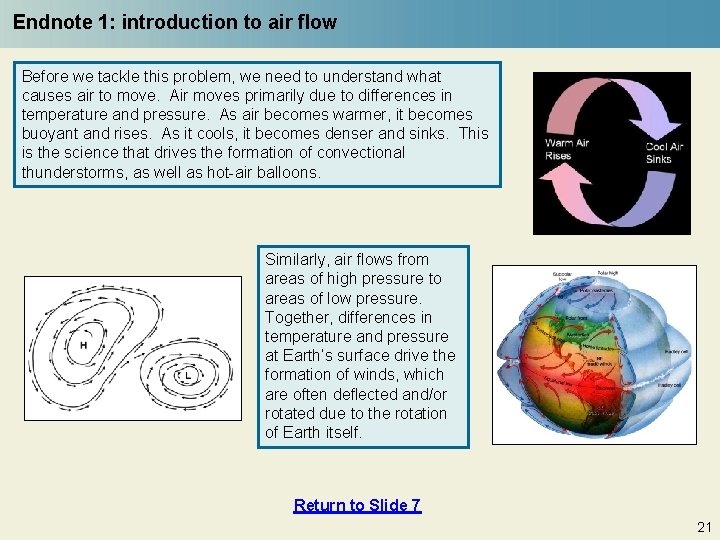
Endnote 1: introduction to air flow Before we tackle this problem, we need to understand what causes air to move. Air moves primarily due to differences in temperature and pressure. As air becomes warmer, it becomes buoyant and rises. As it cools, it becomes denser and sinks. This is the science that drives the formation of convectional thunderstorms, as well as hot-air balloons. Similarly, air flows from areas of high pressure to areas of low pressure. Together, differences in temperature and pressure at Earth’s surface drive the formation of winds, which are often deflected and/or rotated due to the rotation of Earth itself. Return to Slide 7 21

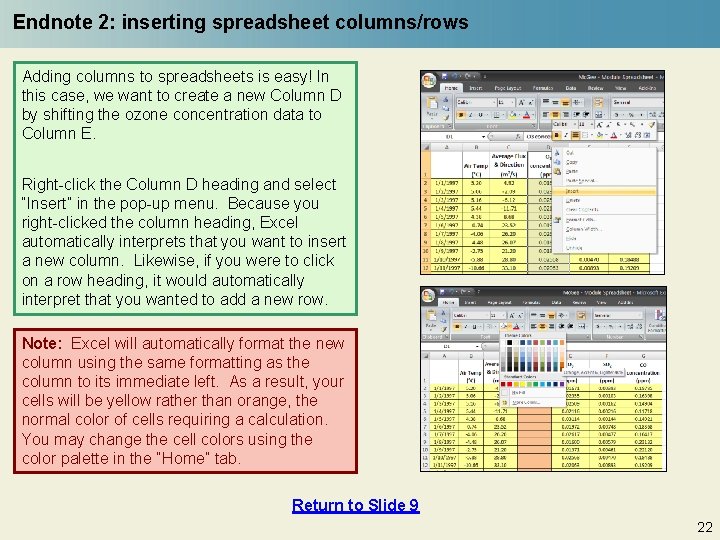
Endnote 2: inserting spreadsheet columns/rows Adding columns to spreadsheets is easy! In this case, we want to create a new Column D by shifting the ozone concentration data to Column E. Right-click the Column D heading and select “Insert” in the pop-up menu. Because you right-clicked the column heading, Excel automatically interprets that you want to insert a new column. Likewise, if you were to click on a row heading, it would automatically interpret that you wanted to add a new row. Note: Excel will automatically format the new column using the same formatting as the column to its immediate left. As a result, your cells will be yellow rather than orange, the normal color of cells requiring a calculation. You may change the cell colors using the color palette in the “Home” tab. Return to Slide 9 22

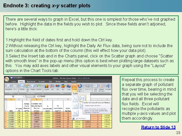
Endnote 3: creating x-y scatter plots There are several ways to graph in Excel, but this one is simplest for those who’ve not graphed before. Highlight the data in the fields you wish to plot. Since these fields aren’t adjoined, here’s a little trick: 1. Highlight the field of dates first and hold down the Ctrl key. 2. Without releasing the Ctrl key, highlight the Daily Air Flux data, being sure not to include the sum calculation at the bottom of the column (this will effect how your data plot). 3. Select the Insert tab and in the Charts panel, click on the Scatter graph and choose “Scatter with smooth lines” in the pop-up menu (this option is best when plotting large datasets such as this. You may add axes labels and other visual elements to your graph using the “Layout” options in the Chart Tools tab. Repeat this process to create a separate graph of pollutant flux over time, bearing in mind that you will be selecting the date and all three pollutant flux fields. Excel will recognize the pollutants as multiple y-axis values and plot them accordingly. Return to Slide 13 23