Learning with Online Constraints Shifting Concepts and Active

Learning with Online Constraints: Shifting Concepts and Active Learning Claire Monteleoni MIT CSAIL Ph. D Thesis Defense August 11 th, 2006 Supervisor: Tommi Jaakkola, MIT CSAIL Committee: Piotr Indyk, MIT CSAIL Sanjoy Dasgupta, UC San Diego

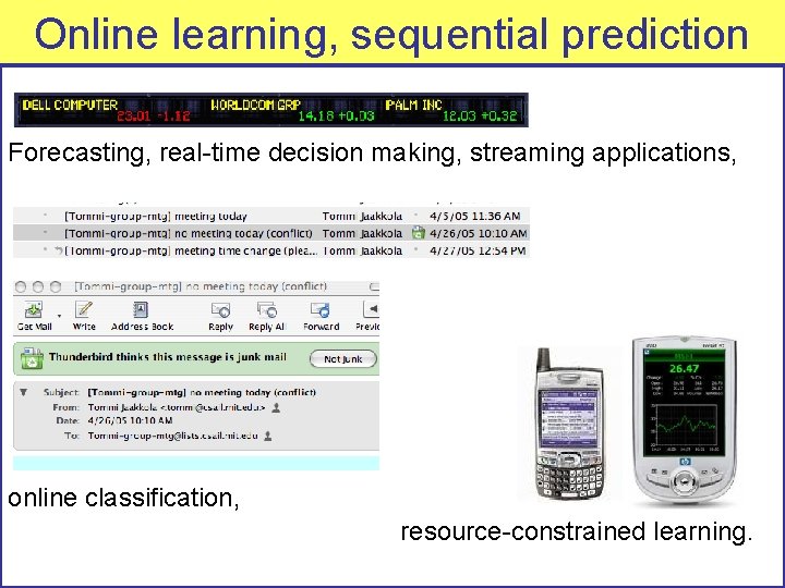
Online learning, sequential prediction Forecasting, real-time decision making, streaming applications, online classification, resource-constrained learning.

Learning with Online Constraints We study learning under these online constraints: 1. Access to the data observations is one-at-a-time only. • Once a data point has been observed, it might never be seen again. • Learner makes a prediction on each observation. ! Models forecasting, temporal prediction problems (internet, stock market, the weather), and high-dimensional streaming data applications 2. Time and memory usage must not scale with data. • Algorithms may not store previously seen data and perform batch learning. ! Models resource-constrained learning, e. g. on small devices

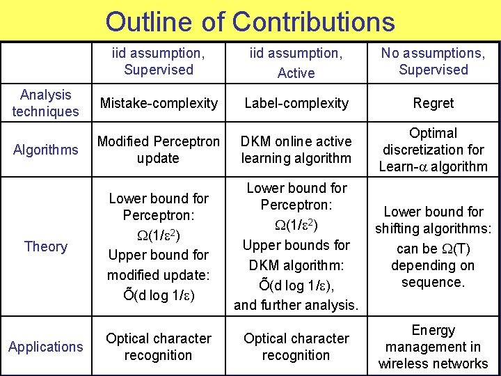
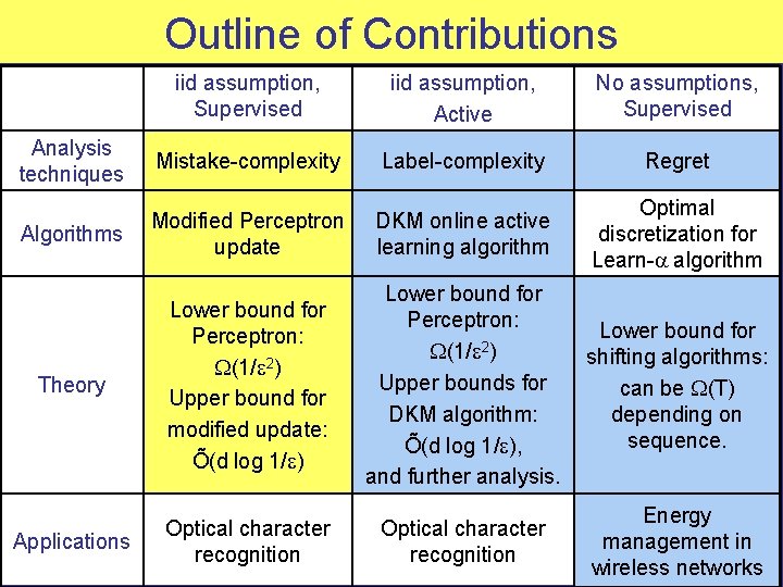
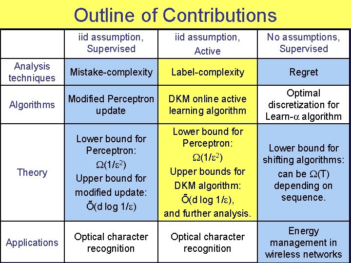
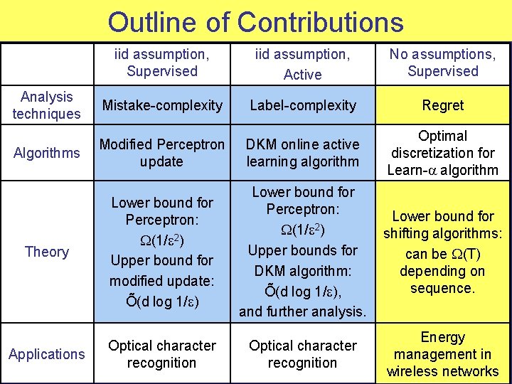
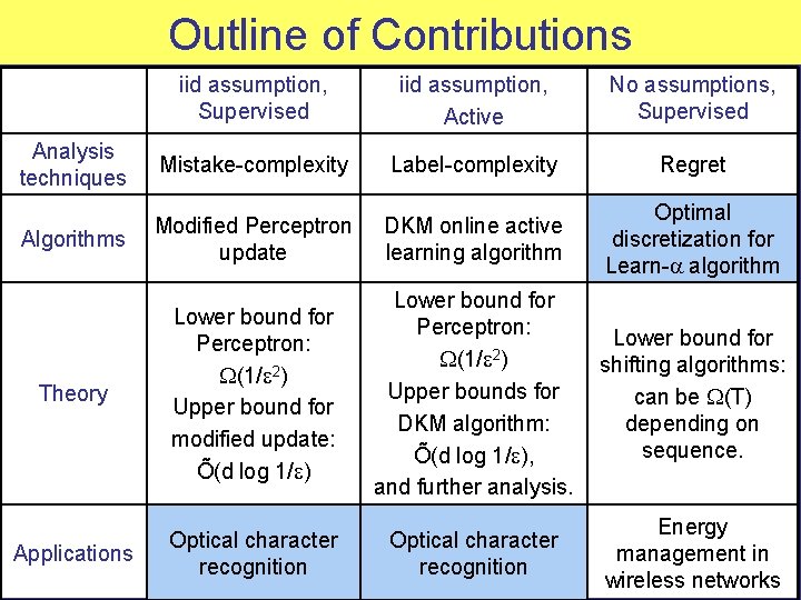
Outline of Contributions iid assumption, Supervised iid assumption, Active No assumptions, Supervised Analysis techniques Mistake-complexity Label-complexity Regret Algorithms Modified Perceptron update DKM online active learning algorithm Optimal discretization for Learn- algorithm Theory Lower bound for Perceptron: (1/ 2) Upper bound for modified update: Õ(d log 1/ ) Lower bound for Perceptron: (1/ 2) Upper bounds for DKM algorithm: Õ(d log 1/ ), and further analysis. Lower bound for shifting algorithms: can be (T) depending on sequence. Applications Optical character recognition Energy management in wireless networks

Outline of Contributions iid assumption, Supervised iid assumption, Active No assumptions, Supervised Analysis techniques Mistake-complexity Label-complexity Regret Algorithms Modified Perceptron update DKM online active learning algorithm Optimal discretization for Learn- algorithm Theory Lower bound for Perceptron: (1/ 2) Upper bound for modified update: Õ(d log 1/ ) Lower bound for Perceptron: (1/ 2) Upper bounds for DKM algorithm: Õ(d log 1/ ), and further analysis. Lower bound for shifting algorithms: can be (T) depending on sequence. Applications Optical character recognition Energy management in wireless networks

Outline of Contributions iid assumption, Supervised iid assumption, Active No assumptions, Supervised Analysis techniques Mistake-complexity Label-complexity Regret Algorithms Modified Perceptron update DKM online active learning algorithm Optimal discretization for Learn- algorithm Theory Lower bound for Perceptron: (1/ 2) Upper bound for modified update: Õ(d log 1/ ) Lower bound for Perceptron: (1/ 2) Upper bounds for DKM algorithm: Õ(d log 1/ ), and further analysis. Lower bound for shifting algorithms: can be (T) depending on sequence. Applications Optical character recognition Energy management in wireless networks

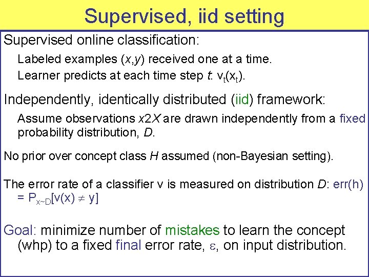
Supervised, iid setting Supervised online classification: Labeled examples (x, y) received one at a time. Learner predicts at each time step t: vt(xt). Independently, identically distributed (iid) framework: Assume observations x 2 X are drawn independently from a fixed probability distribution, D. No prior over concept class H assumed (non-Bayesian setting). The error rate of a classifier v is measured on distribution D: err(h) = Px~D[v(x) y] Goal: minimize number of mistakes to learn the concept (whp) to a fixed final error rate, , on input distribution.

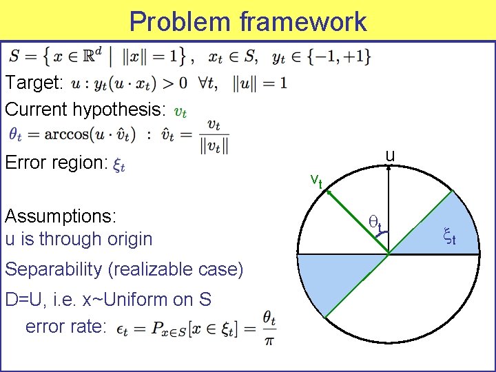
Problem framework Target: Current hypothesis: Error region: Assumptions: u is through origin Separability (realizable case) D=U, i. e. x~Uniform on S error rate: u vt t t

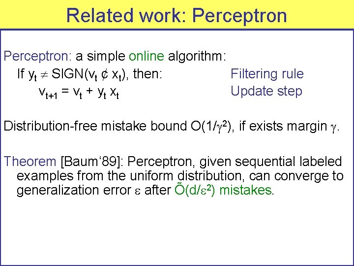
Related work: Perceptron: a simple online algorithm: If yt SIGN(vt ¢ xt), then: Filtering rule vt+1 = vt + yt xt Update step Distribution-free mistake bound O(1/ 2), if exists margin . Theorem [Baum‘ 89]: Perceptron, given sequential labeled examples from the uniform distribution, can converge to generalization error after Õ(d/ 2) mistakes.

Contributions in supervised, iid case [Dasgupta, Kalai & M, COLT 2005] A lower bound on mistakes for Perceptron of (1/ 2). A modified Perceptron update with a Õ(d log 1/ ) mistake bound.

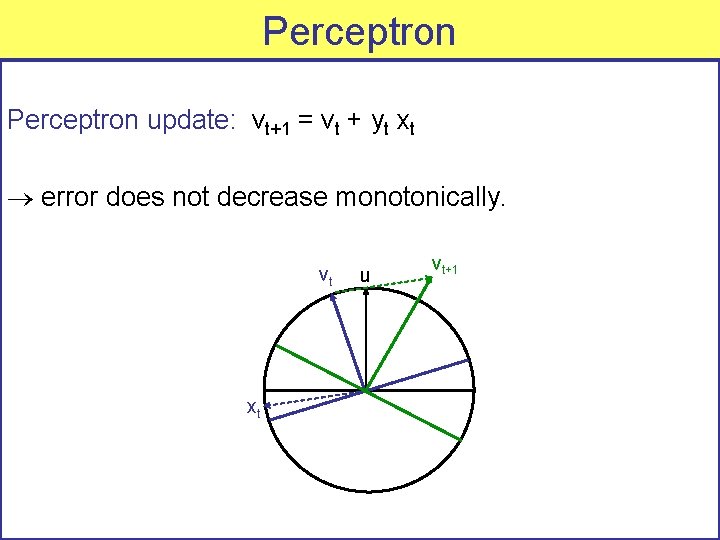
Perceptron update: vt+1 = vt + yt xt error does not decrease monotonically. vt xt u vt+1

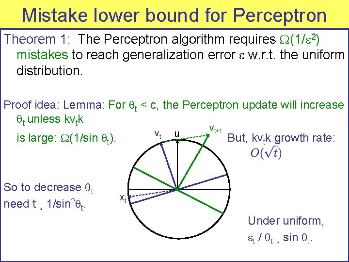
Mistake lower bound for Perceptron Theorem 1: The Perceptron algorithm requires (1/ 2) mistakes to reach generalization error w. r. t. the uniform distribution. Proof idea: Lemma: For t < c, the Perceptron update will increase t unless kvtk vt is large: (1/sin t). So to decrease t need t ¸ 1/sin 2 t. u vt+1 But, kvtk growth rate: xt Under uniform, t / t ¸ sin t.

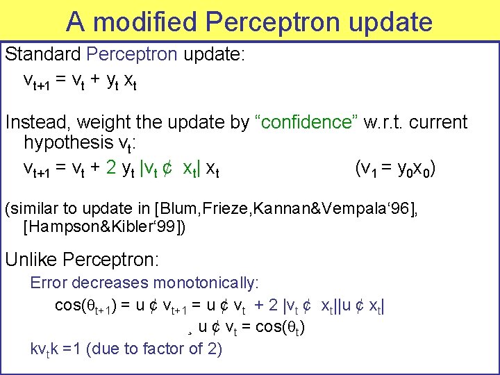
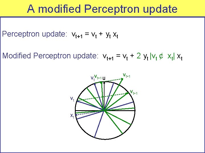
A modified Perceptron update Standard Perceptron update: vt+1 = vt + yt xt Instead, weight the update by “confidence” w. r. t. current hypothesis vt: vt+1 = vt + 2 yt |vt ¢ xt| xt (v 1 = y 0 x 0) (similar to update in [Blum, Frieze, Kannan&Vempala‘ 96], [Hampson&Kibler‘ 99]) Unlike Perceptron: Error decreases monotonically: cos( t+1) = u ¢ vt+1 = u ¢ vt + 2 |vt ¢ xt||u ¢ xt| ¸ u ¢ vt = cos( t) kvtk =1 (due to factor of 2)

A modified Perceptron update: vt+1 = vt + yt xt Modified Perceptron update: vt+1 = vt + 2 yt |vt ¢ xt| xt vtvt+1 u vt xt vt+1

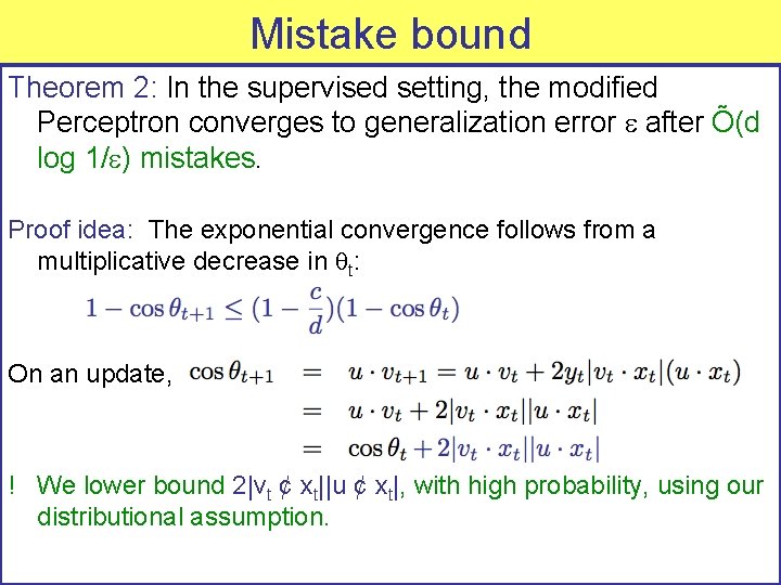
Mistake bound Theorem 2: In the supervised setting, the modified Perceptron converges to generalization error after Õ(d log 1/ ) mistakes. Proof idea: The exponential convergence follows from a multiplicative decrease in t: On an update, ! We lower bound 2|vt ¢ xt||u ¢ xt|, with high probability, using our distributional assumption.

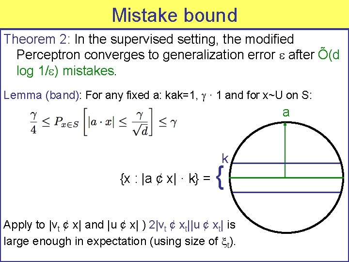
Mistake bound Theorem 2: In the supervised setting, the modified Perceptron converges to generalization error after Õ(d log 1/ ) mistakes. Lemma (band): For any fixed a: kak=1, · 1 and for x~U on S: a k {x : |a ¢ x| · k} = { Apply to |vt ¢ x| and |u ¢ x| ) 2|vt ¢ xt||u ¢ xt| is large enough in expectation (using size of t).

Outline of Contributions iid assumption, Supervised iid assumption, Active No assumptions, Supervised Analysis techniques Mistake-complexity Label-complexity Regret Algorithms Modified Perceptron update DKM online active learning algorithm Optimal discretization for Learn- algorithm Theory Lower bound for Perceptron: (1/ 2) Upper bound for modified update: Õ(d log 1/ ) Lower bound for Perceptron: (1/ 2) Upper bounds for DKM algorithm: Õ(d log 1/ ), and further analysis. Lower bound for shifting algorithms: can be (T) depending on sequence. Applications Optical character recognition Energy management in wireless networks

Active learning Machine learning applications, e. g. Medical diagnosis Document/webpage classification Speech recognition Unlabeled data is abundant, but labels are expensive. Active learning is a useful model here. Allows for intelligent choices of which examples to label. Label-complexity: the number of labeled examples required to learn via active learning. ! can be much lower than the PAC sample complexity!

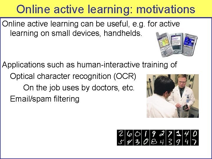
Online active learning: motivations Online active learning can be useful, e. g. for active learning on small devices, handhelds. Applications such as human-interactive training of Optical character recognition (OCR) On the job uses by doctors, etc. Email/spam filtering

PAC-like Onlineselective active learning sampling framework Selective sampling [Cohn, Atlas&Ladner 92]: Given: stream (or pool) of unlabeled examples, x 2 X, drawn i. i. d. from input distribution, D over X. Learner may request labels on examples in the stream/pool. (Noiseless) o� racle access to correct labels, y 2 Y. Constant cost per label The error rate of any classifier v is measured on distribution D: err(h) = Px~D[v(x) y] PAC-like case: no prior on hypotheses assumed (non-Bayesian). Goal: minimize number of labels to learn the concept (whp) to a fixed final error rate, , on input distribution. We impose online constraints on time and memory.

Measures of complexity PAC sample complexity: Supervised setting: number of (labeled) examples, sampled iid from D, to reach error rate . Mistake-complexity: Supervised setting: number of mistakes to reach error rate Label-complexity: Active setting: number of label queries to reach error rate Error complexity: Total prediction errors made on (labeled and/or unlabeled) examples, before reaching error rate Supervised setting: equal to mistake-complexity. Active setting: mistakes are a subset of total errors on which learner queries a label.

Related work: Query by Committee Analysis under selective sampling model, of Query By Committee algorithm [Seung, Opper&Sompolinsky‘ 92] : Theorem [Freund, Seung, Shamir&Tishby ‘ 97]: Under Bayesian assumptions, when selective sampling from the uniform, QBC can learn a half-space through the origin to generalization error , using Õ(d log 1/ ) labels. ! But not online: space required, and time complexity of the update both scale with number of seen mistakes!

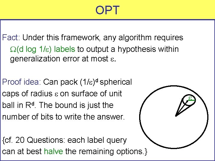
OPT Fact: Under this framework, any algorithm requires (d log 1/ ) labels to output a hypothesis within generalization error at most Proof idea: Can pack (1/ )d spherical caps of radius on surface of unit ball in Rd. The bound is just the number of bits to write the answer. {cf. 20 Questions: each label query can at best halve the remaining options. }

Contributions for online active learning [Dasgupta, Kalai & M, COLT 2005] A lower bound for Perceptron in active learning context, paired with any active learning rule, of (1/ 2) labels. An online active learning algorithm and a label bound of Õ(d log 1/ ). A bound of Õ(d log 1/ ) on total errors (labeled or unlabeled). [M, 2006] Further analyses, including a label bound for DKM of Õ(poly(1/ d log 1/ ) under -similar to uniform distributions.

Lower bound on labels for Perceptron Corollary 1: The Perceptron algorithm, using any active learning rule, requires (1/ 2) labels to reach generalization error w. r. t. the uniform distribution. Proof: Theorem 1 provides a (1/ 2) lower bound on updates. A label is required to identify each mistake, and updates are only performed on mistakes.

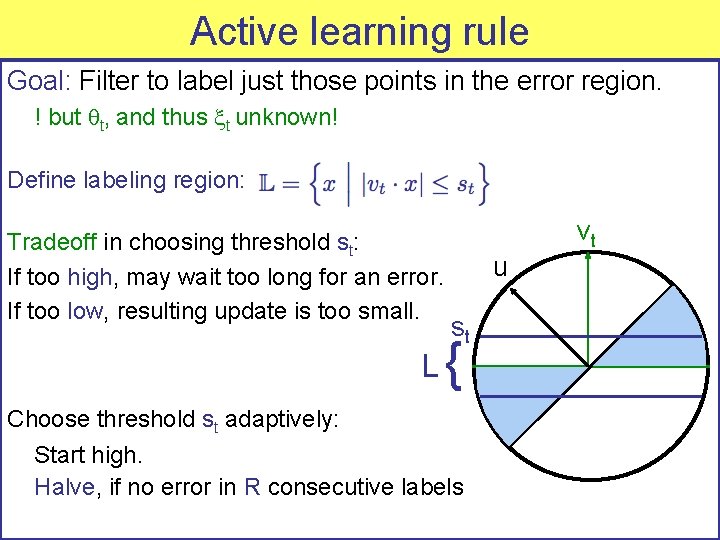
Active learning rule Goal: Filter to label just those points in the error region. ! but t, and thus t unknown! Define labeling region: Tradeoff in choosing threshold st: If too high, may wait too long for an error. If too low, resulting update is too small. L vt u st { Choose threshold st adaptively: Start high. Halve, if no error in R consecutive labels

Label bound Theorem 3: In the active learning setting, the modified Perceptron, using the adaptive filtering rule, will converge to generalization error after Õ(d log 1/ ) labels. Corollary: The total errors (labeled and unlabeled) will be Õ(d log 1/ ).

Proof technique Proof outline: We show the following lemmas hold with sufficient probability: Lemma 1. st does not decrease too quickly: Lemma 2. We query labels on a constant fraction of t. Lemma 3. With constant probability the update is good. By algorithm, ~1/R labels are updates. 9 R = Õ(1). ) Can thus bound labels and total errors by mistakes.

Related work Negative results: • Homogenous linear separators under arbitrary distributions and non-homogeneous under uniform: (1/ ) [Dasgupta‘ 04]. • Arbitrary (concept, distribution)-pairs that are “ -splittable”: (1/ [Dasgupta‘ 05]. • Agnostic setting where best in class has generalization error : ( 2/ 2) [Kääriäinen‘ 06]. Upper bounds on label-complexity for intractable schemes: • General concepts and input distributions, realizable [D‘ 05]. • Linear separators under uniform, an agnostic scenario: Õ(d 2 log 1/ ) [Balcan, Beygelzimer&Langford‘ 06]. Algorithms analyzed in other frameworks: • Individual sequences: [Cesa-Bianchi, Gentile&Zaniboni‘ 04]. • Bayesian assumption: linear separators under the uniform, realizable case, using QBC [SOS‘ 92], Õ(d log 1/ ) [FSST‘ 97].

[DKM 05] in context samples PAC complexity [Long‘ 03] [Long‘ 95] Perceptron [Baum‘ 97] mistakes labels total errors online? Õ(d/ ) Õ(d/ 3) (1/ 2) Õ(d/ 2) (1/ 2) p (1/ 2) CAL [BBL‘ 06] Õ((d 2/ Õ(d 2 log 1/ ) QBC [FSST‘ 97] Õ(d/ log 1/ ) Õ(d log 1/ ) X X p [DKM‘ 05] Õ(d/ log 1/ ) Õ(d log 1/ )

Further analysis: version space Vt is set of hypotheses in concept class still consistent with all t labeled examples seen. Theorem 4: There exists a linearly separable sequence of t examples such that running DKM on will yield a hypothesis vt that misclassifies a data point x 2 . ) DKM’s hypothesis need not be in version space. This motivates target region approach: Define pseudo-metric d(h, h’) = Px » D [h(x) h’(x)] Target region H* = Bd(u, ) {Reached by DKM after Õ(d log 1/ ) labels} V 1 = Bd(u, ) µ H*, however: Lemma(s): For any finite t, neither Vt µ H* nor H*µ Vt need hold.

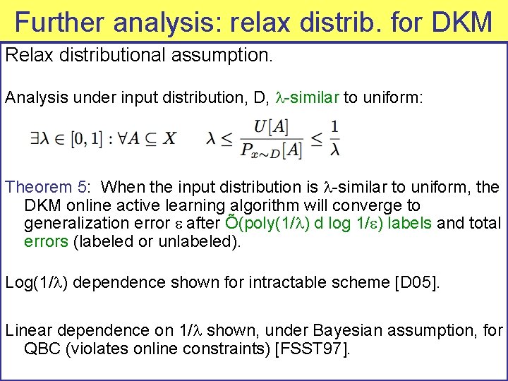
Further analysis: relax distrib. for DKM Relax distributional assumption. Analysis under input distribution, D, -similar to uniform: Theorem 5: When the input distribution is -similar to uniform, the DKM online active learning algorithm will converge to generalization error after Õ(poly(1/ ) d log 1/ ) labels and total errors (labeled or unlabeled). Log(1/ ) dependence shown for intractable scheme [D 05]. Linear dependence on 1/ shown, under Bayesian assumption, for QBC (violates online constraints) [FSST 97].

Outline of Contributions iid assumption, Supervised iid assumption, Active No assumptions, Supervised Analysis techniques Mistake-complexity Label-complexity Regret Algorithms Modified Perceptron update DKM online active learning algorithm Optimal discretization for Learn- algorithm Theory Lower bound for Perceptron: (1/ 2) Upper bound for modified update: Õ(d log 1/ ) Lower bound for Perceptron: (1/ 2) Upper bounds for DKM algorithm: Õ(d log 1/ ), and further analysis. Lower bound for shifting algorithms: can be (T) depending on sequence. Applications Optical character recognition Energy management in wireless networks

Non-stochastic setting Remove all statistical assumptions. No assumptions on observation sequence. E. g. , observations can even be generated online by an adaptive adversary. Framework models supervised learning: Regression, estimation or classification. Many prediction loss functions: - many concept classes - problem need not be realizable Analyze regret: difference in cumulative prediction loss from that of the optimal (in hind-sight) comparator algorithm for the particular sequence observed.

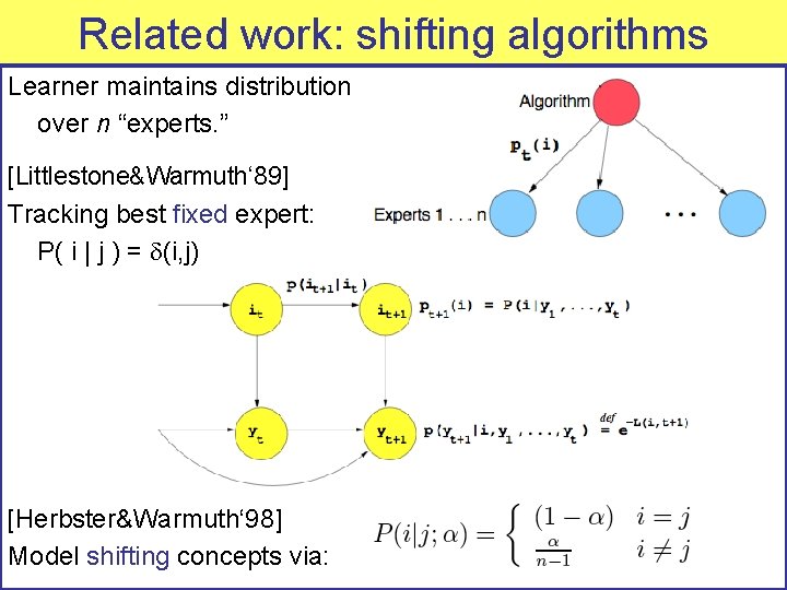
Related work: shifting algorithms Learner maintains distribution over n “experts. ” [Littlestone&Warmuth‘ 89] Tracking best fixed expert: P( i | j ) = (i, j) [Herbster&Warmuth‘ 98] Model shifting concepts via:

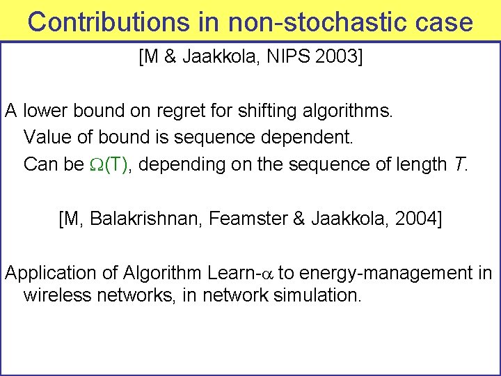
Contributions in non-stochastic case [M & Jaakkola, NIPS 2003] A lower bound on regret for shifting algorithms. Value of bound is sequence dependent. Can be (T), depending on the sequence of length T. [M, Balakrishnan, Feamster & Jaakkola, 2004] Application of Algorithm Learn- to energy-management in wireless networks, in network simulation.

Review of our previous work [M, 2003] [M & Jaakkola, NIPS 2003] Upper bound on regret for Learn- algorithm of O(log T). Learn- algorithm: Track best expert: shifting sub-algorithm (each running with different value).

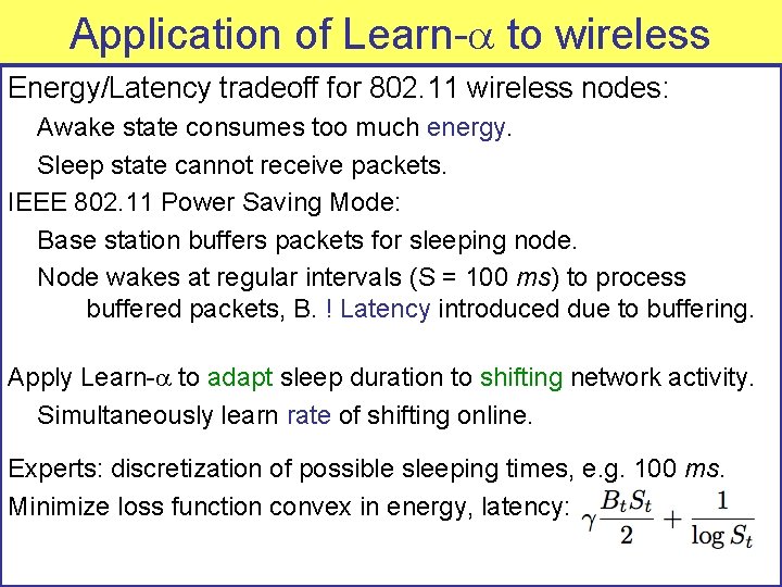
Application of Learn- to wireless Energy/Latency tradeoff for 802. 11 wireless nodes: Awake state consumes too much energy. Sleep state cannot receive packets. IEEE 802. 11 Power Saving Mode: Base station buffers packets for sleeping node. Node wakes at regular intervals (S = 100 ms) to process buffered packets, B. ! Latency introduced due to buffering. Apply Learn- to adapt sleep duration to shifting network activity. Simultaneously learn rate of shifting online. Experts: discretization of possible sleeping times, e. g. 100 ms. Minimize loss function convex in energy, latency:

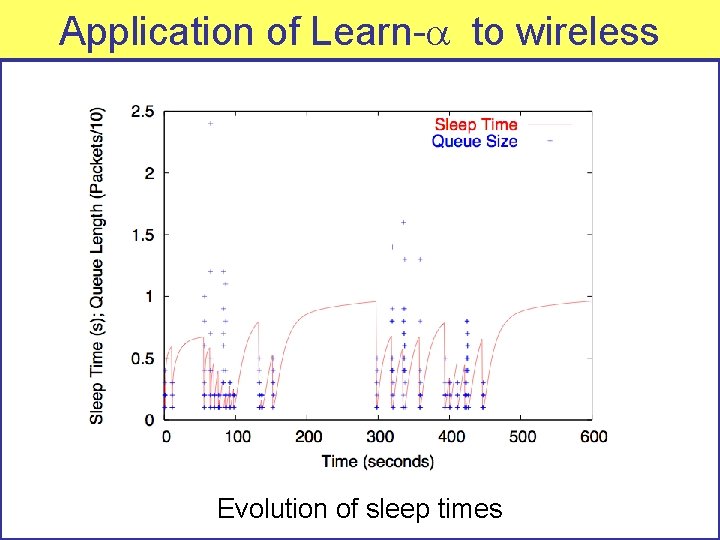
Application of Learn- to wireless Evolution of sleep times

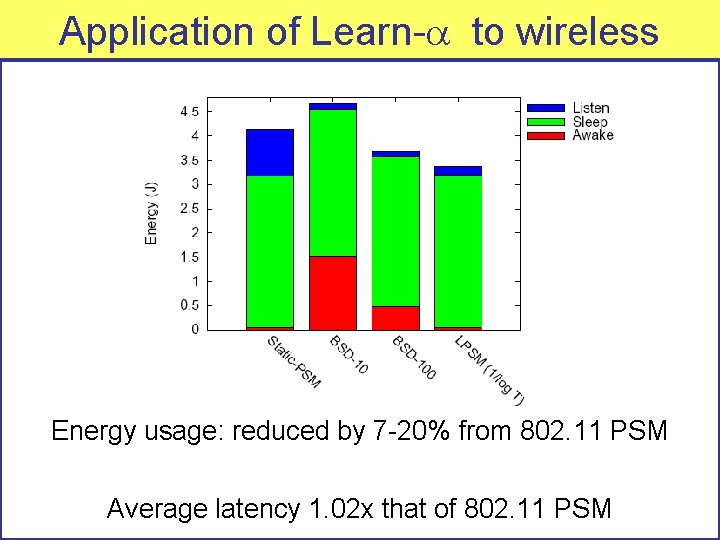
Application of Learn- to wireless Energy usage: reduced by 7 -20% from 802. 11 PSM Average latency 1. 02 x that of 802. 11 PSM

Outline of Contributions iid assumption, Supervised iid assumption, Active No assumptions, Supervised Analysis techniques Mistake-complexity Label-complexity Regret Algorithms Modified Perceptron update DKM online active learning algorithm Optimal discretization for Learn- algorithm Theory Lower bound for Perceptron: (1/ 2) Upper bound for modified update: Õ(d log 1/ ) Lower bound for Perceptron: (1/ 2) Upper bounds for DKM algorithm: Õ(d log 1/ ), and further analysis. Lower bound for shifting algorithms: can be (T) depending on sequence. Applications Optical character recognition Energy management in wireless networks

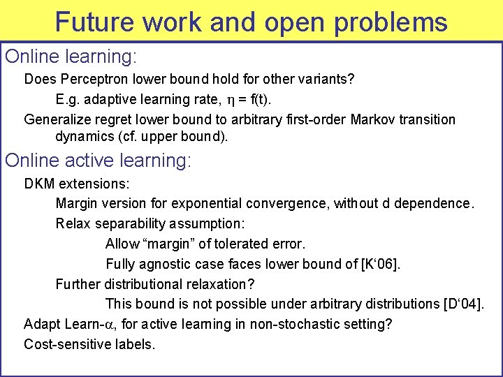
Future work and open problems Online learning: Does Perceptron lower bound hold for other variants? E. g. adaptive learning rate, = f(t). Generalize regret lower bound to arbitrary first-order Markov transition dynamics (cf. upper bound). Online active learning: DKM extensions: Margin version for exponential convergence, without d dependence. Relax separability assumption: Allow “margin” of tolerated error. Fully agnostic case faces lower bound of [K‘ 06]. Further distributional relaxation? This bound is not possible under arbitrary distributions [D‘ 04]. Adapt Learn- , for active learning in non-stochastic setting? Cost-sensitive labels.

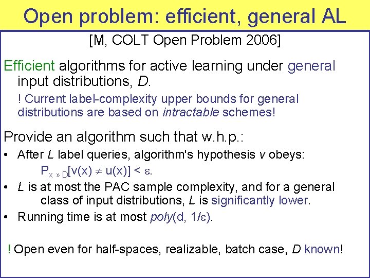
Open problem: efficient, general AL [M, COLT Open Problem 2006] Efficient algorithms for active learning under general input distributions, D. ! Current label-complexity upper bounds for general distributions are based on intractable schemes! Provide an algorithm such that w. h. p. : • After L label queries, algorithm's hypothesis v obeys: Px » D[v(x) u(x)] < . • L is at most the PAC sample complexity, and for a general class of input distributions, L is significantly lower. • Running time is at most poly(d, 1/ ). ! Open even for half-spaces, realizable, batch case, D known!

Thank you! And many thanks to: Advisor: Tommi Jaakkola Committee: Sanjoy Dasgupta, Piotr Indyk Coauthors: Hari Balakrishnan, Sanjoy Dasgupta, Nick Feamster, Tommi Jaakkola, Adam Tauman Kalai, Matti Kääriäinen Numerous colleagues and friends. My family!