Space Research Institute of Russian Academy of Sciences

Space Research Institute of Russian Academy of Sciences Terrestrial bow shock analytical global modeling M. Verigin Talk to workshop: Solar - Terrestrial Interactions from Microscale to Global Models Sinaia, Romania, September 6 -10, 2005

Terrestrial bow shock analytical global modeling Introduction A large number of observations of shocks and shock-related phenomena at different planets require robust and convenient BS model for data classification and analysis, e. g. , • Exploration of electron and ion foreshock formation • Studies of plasma wave generation by specularly and diffusely reflected ions • Investigations of mechanisms of the solar wind deceleration in the shock foot and shock itself • Studies of the plasma wave propagation along shock surfaces • Analyses of the processes of shock overshoot formation and plasma turbulence generation inside the magnetosheath • Investigation of micropulsations generated at the bow shock and magnetopause, etc. Huge uniform databases recently appeared with Earth’s BS crossings by: IMP-8 (1977 -01 -01 - 2000 -06 -09) Geotail (1995 -01 -01 - 1997 -11 -02) Magion-4 (1996 -02 -01 - 1997 -07 -31) Cluster (2001 -02 -02 - 2002 -05 -20) http: //nssdc. gsfc. nasa. gov/ftphelper/bowshock. htm http: //spdf. gsfc. nasa. gov/bowshock/

Terrestrial bow shock analytical global modeling Introduction Theoretical BS models provide a reliable baseline for bow shock related studies. These are: • gasdynamic (GD), or • magnetohydrodynamic (MHD), or • semikinetic (hybrid) particle simulations e. g. , Spreiter et al. , 1966; Cairns & Lyon, 1995; Tanaka, 1995; Kabin et al. , 2000; Brecht, 1997… Theoretical approaches, especially the last two, • require sophisticated, non-transparent numerical codes and • plenty of processor time for even a single run on modern supercomputers. They are presently inconvenient for wide use, and practically impossible to be used for the bow shock position and shape tracing with high time resolution.

Terrestrial bow shock analytical global modeling Introduction Empirical models are used for most of shock related studies: e. g. , Fairfield, 1971; Formisano, 1979 Slavin and Holzer, 1981 Nĕmeček & Šafránková, 1991 Peredo et al. , 1995; Chao et al. , 2002 Chapman and Cairns, 2003 Though providing general description of the average shape and position of the bow shock, these models generally • have uncertain limits of applicability • fail for unusual solar wind conditions • use conic sections for description of bow shock shape • do not provide correct asymptotic behavior and • do not consider the influence of specific heat ratio on the planetary bow shock position Maximal use of exact analytical theoretical relations is highly welcomed for reasonable parameterization of accurate numerical BS modeling – so called semi-empirical modeling approach.

Magnetopause shape parameterization e. g. detailed GD tables by Lyubimov & Rusanov [1970] r 0 – obstacle nose position R 0 – nose radius of curvature b 0 – obstacle ‘bluntness’ Obstacle shape: b 0 < -1 - blunt elliptic b 0 = -1 - spherical -1 < b 0 < 0 - elongated elliptic b 0 = 0 - parabolic b 0 > 0 - hyperbolic Different equations for magnetopause shapes Holzer & Slavin [1978 r = l/(1+ cos ) r 0 = l/(1+ ) Roelof & Sibeck [1993] y 2+ax 2+bx+c=0 ar 02+br 0+c=0 Petrinec &Russell [1996] r = r 0(1+ )/(1+ cos ) R 0 = l b 0 = 2 -1 R 0 = ar 0+b/2 b 0 = -a r 0 R 0 = r 0(1+ ) b 0 = 2 -1 Kawano al. [1998], x = (r 0 -x 0)(1+ )cos /(1+ cos )+x 0 parametric, - parameter y = (r 0 -x 0)(1+ )sin /(1+ cos ) r 0 R 0 = (r 0 -x 0)(1+ ) b 0 = 2 -1 Kuznetsov & Yushkov [2000] x = r 0 – gy 2 r 0 R 0 = 1/(2 g) R 0 =2 r 0/(2 - ) Shue et al. [2000] r = r 0(2/(1+cos )) r 0 Spreiter et al. [1966] pressure balanced p(r) = p(r 0) (r 0/r)6 r 0 Spreiter et al. [1970] Verigin et al. [1997] pressure balanced p(r) = p(r 0)exp((r 0 -r)/H) pressure balanced p(r) = p(r 0) [(1 - ) (r 0/r)6 + exp((r 0 -r)/H)] r 0 b 0 =(6 -8)( -1)/( -2)3

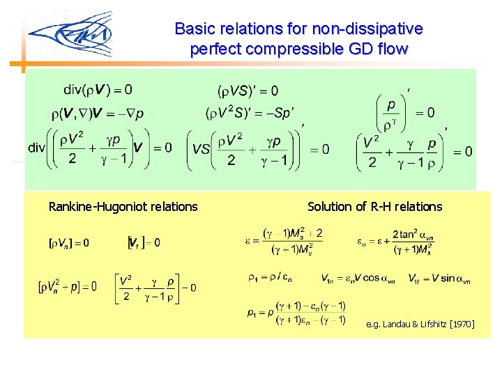
Basic relations for non-dissipative perfect compressible GD flow Rankine-Hugoniot relations Solution of R-H relations e. g. Landau & Lifshitz [1970]

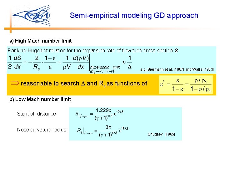
Semi-empirical modeling GD approach a) High Mach number limit Rankine-Hugoniot relation for the expansion rate of flow tube cross-section S e. g. Biermann et al. [1967] and Wallis [1973] reasonable to search and Rs as functions of b) Low Mach number limit Standoff distance Nose curvature radius Shugaev [1965]

Empiric relations for BS stand off distance Reference Relation Specific feature Comment Serbin [1958] b 0 = -1 , but with incorrect power Ambrosio & Wortman [1962] b 0 = -1 , but with incorrect power Seiff [1962] b 0 = -1 , unrealistic Hida [1955], Shugaev [1964] b 0 - unspecified correct power of Spreiter et al. [1966] , unrealistic Farris & Russell [1994] , but with incorrect power b 0 = -1 , unrealistic, but wide region of applicability - < b 0 < -0. 25 same advantages and disadvan – tages, but describes dependency on bo also b 0 - unspecified , with correct power Minailos [1973] See below the table*) Verigin et al. [1997] *)

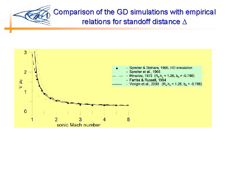
Comparison of the GD simulations with empirical relations for standoff distance

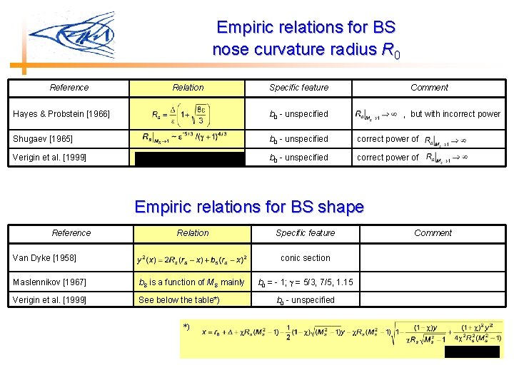
Empiric relations for BS nose curvature radius R 0 Reference Relation Specific feature Comment Hayes & Probstein [1966] b 0 - unspecified , but with incorrect power Shugaev [1965] b 0 - unspecified correct power of Verigin et al. [1999] b 0 - unspecified correct power of Empiric relations for BS shape Reference Relation Van Dyke [1958] Specific feature conic section Maslennikov [1967] b. S is a function of MS mainly Verigin et al. [1999] See below the table*) *) b 0 = - 1; = 5/3, 7/5, 1. 15 b 0 - unspecified Comment

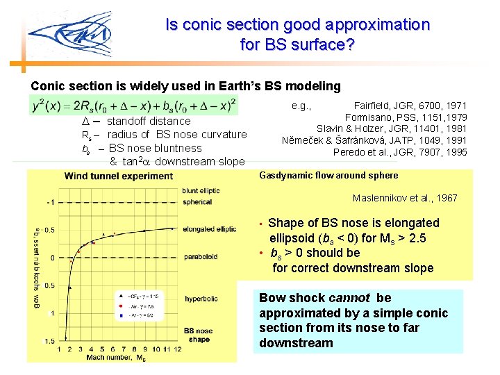
Is conic section good approximation for BS surface? Conic section is widely used in Earth’s BS modeling – standoff distance Rs – radius of BS nose curvature bs – BS nose bluntness & tan 2 downstream slope e. g. , Fairfield, JGR, 6700, 1971 Formisano, PSS, 1151, 1979 Slavin & Holzer, JGR, 11401, 1981 Nĕmeček & Šafránková, JATP, 1049, 1991 Peredo et al. , JGR, 7907, 1995 Gasdynamic flow around sphere Maslennikov et al. , 1967 • Shape of BS nose is elongated ellipsoid (bs < 0) for Ms > 2. 5 • bs > 0 should be for correct downstream slope Bow shock cannot be approximated by a simple conic section from its nose to far downstream

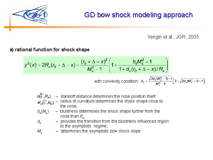
GD bow shock modeling approach Verigin et al. , JGR, 2003 a) rational function for shock shape with convexity condition: – standoff distance determines the nose position itself; – radius of curvature determines the shock shape close to the nose; bs(Ms) – bluntness determines the shock shape further from the nose than Rs; ds – provides the transition from the bluntness influenced region to the asymptotic regime; Ms – determines the asymptotic bow shock slope

GD bow shock modeling approach Verigin et al. , JGR, 2003

Basic dependencies of , Rs, bs, ds on Ms and b 0 for = 7/5

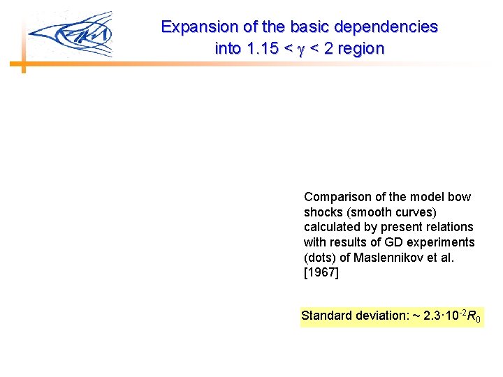
Expansion of the basic dependencies into 1. 15 < < 2 region Comparison of the model bow shocks (smooth curves) calculated by present relations with results of GD experiments (dots) of Maslennikov et al. [1967] Standard deviation: ~ 2. 3· 10 -2 R 0

Expansion of the basic dependencies into 1. 15 < < 2 region

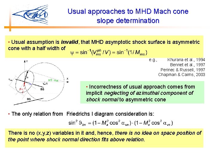
Usual approaches to MHD Mach cone slope determination • Usual assumption is invalid, that MHD asymptotic shock surface is asymmetric cone with a half width of e. g. , Khurana et al. , 1994 Bennet et al. , 1997 Perinec & Russell, 1997 Chapman & Cairns, 2003 • Incorrectness of usual approach comes from implicit neglecting of azimuthal component of shock normal to asymmetric cone • The only relation from Friedrichs I diagram consideration is: There is no (x, y, z) variables in it and, hence, there is no idea on space position of the point where shock normal direction fits above relation.

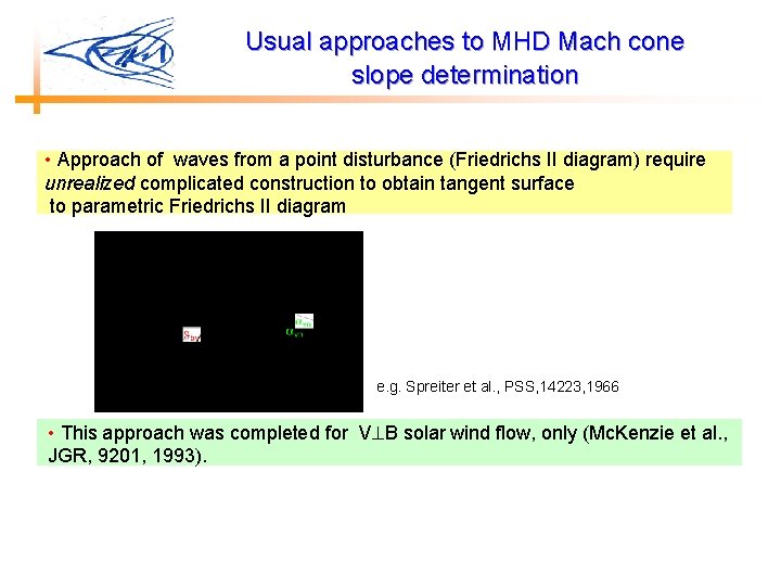
Usual approaches to MHD Mach cone slope determination • Approach of waves from a point disturbance (Friedrichs II diagram) require unrealized complicated construction to obtain tangent surface to parametric Friedrichs II diagram e. g. Spreiter et al. , PSS, 14223, 1966 • This approach was completed for V B solar wind flow, only (Mc. Kenzie et al. , JGR, 9201, 1993).

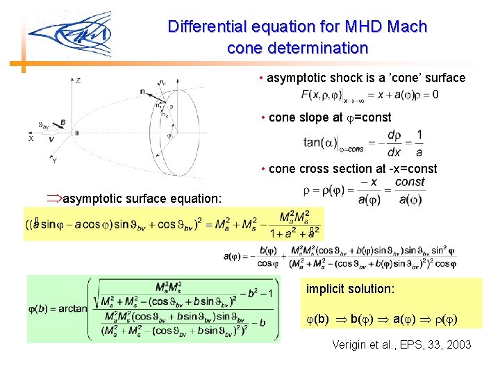
Differential equation for MHD Mach cone determination • asymptotic shock is a ’cone’ surface • cone slope at =const • cone cross section at -x=const asymptotic surface equation: implicit solution: (b) b( ) a( ) Verigin et al. , EPS, 33, 2003

Exact analytic solution for distant BS cross-section Cross-section of the fast (smooth curve), slow (triangle-like features) shocks, and of Alfven wings (asterisks) discontinuities far downstream of the obstacle. Dashed circle - minimal possible slope of the fast shock Dot-dashed circle - maximal possible slope of the fast shock

Exact analytic solution for distant BS cross-section V B solar wind flow – ‘kindersurprise’ cross-section

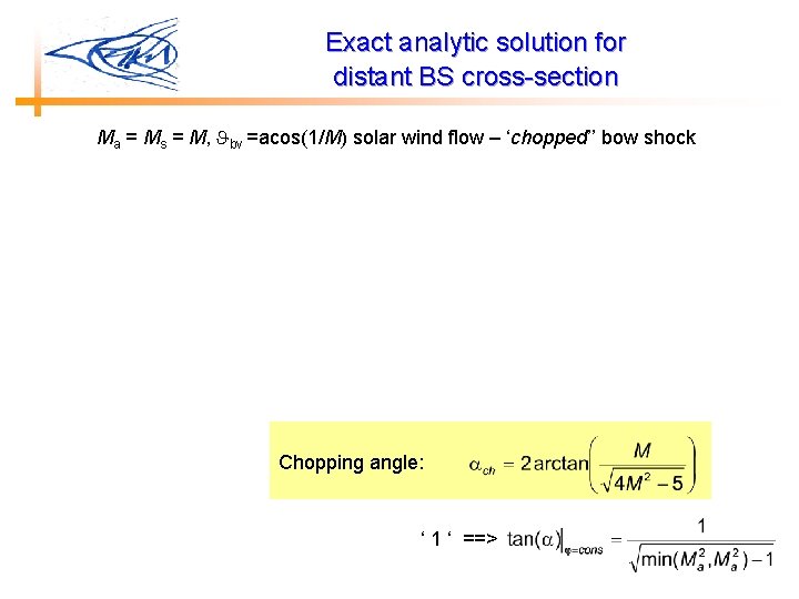
Exact analytic solution for distant BS cross-section Ma = Ms = M, bv =acos(1/M) solar wind flow – ‘chopped’’ bow shock Chopping angle: ‘ 1 ‘ ==>

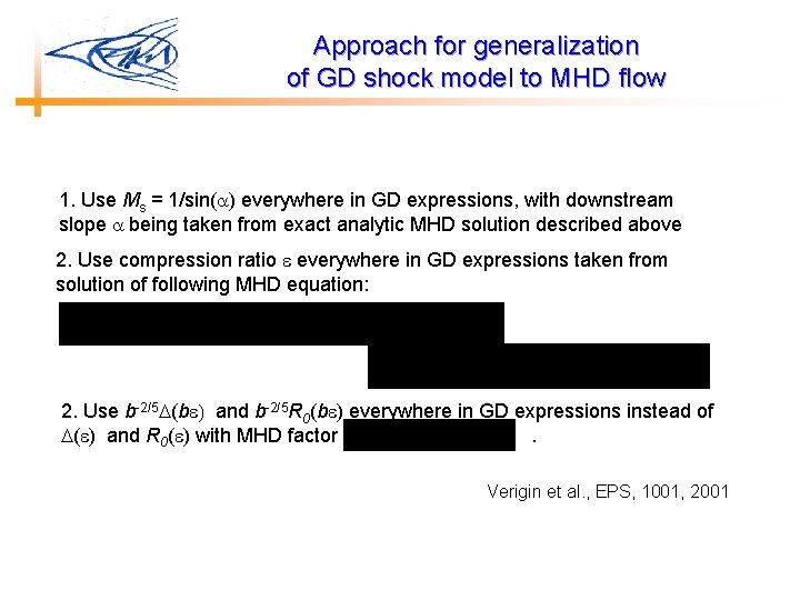
Approach for generalization of GD shock model to MHD flow 1. Use Ms = 1/sin( ) everywhere in GD expressions, with downstream slope being taken from exact analytic MHD solution described above 2. Use compression ratio everywhere in GD expressions taken from solution of following MHD equation: 2. Use b-2/5 (b ) and b-2/5 R 0(b ) everywhere in GD expressions instead of ( ) and R 0( ) with MHD factor . Verigin et al. , EPS, 1001, 2001

Examples of variations of modeled BS relative to Wind position

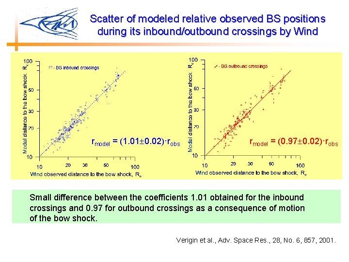
Scatter of modeled relative observed BS positions during its inbound/outbound crossings by Wind rmodel = (1. 01 0. 02)·robs rmodel = (0. 97 0. 02)·robs Small difference between the coefficients 1. 01 obtained for the inbound crossings and 0. 97 for outbound crossings as a consequence of motion of the bow shock. Verigin et al. , Adv. Space Res. , 28, No. 6, 857, 2001.

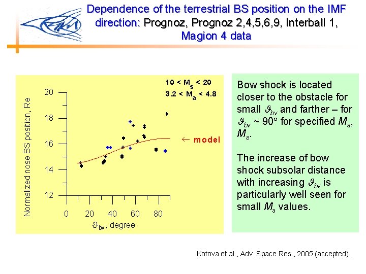
Dependence of the terrestrial BS position on the IMF direction: Prognoz, Prognoz 2, 4, 5, 6, 9, Interball 1, Magion 4 data 10 < M < 20 s Normalized nose BS position, Re 20 3. 2 < M < 4. 8 a 18 ¬ m odel 16 14 12 0 20 40 60 bv, degree 80 Bow shock is located closer to the obstacle for small bv and farther – for bv ~ 90 for specified Ma, Ms. The increase of bow shock subsolar distance with increasing bv is particularly well seen for small Ma values. Kotova et al. , Adv. Space Res. , 2005 (accepted).

Bow shock approach to Earth with decreasing of Ma in field aligned flows according to INTERBALL/Magion 4 observations Verigin et al. , Adv. Space Res. , 28, No. 6, 857, 2001.

Earth’s bow shock terminator anisotropy as seen from Wind observations analysis Verigin et al. , EPS, 1001, 2001

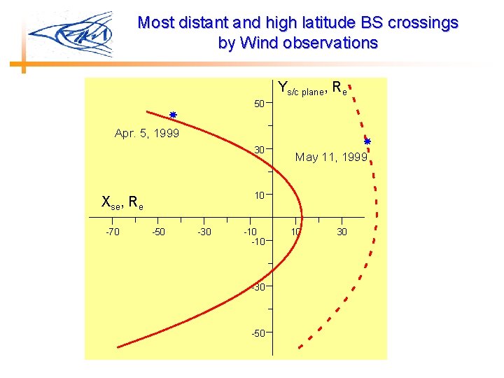
Most distant and high latitude BS crossings by Wind observations Ys/c plane, Re 50 Apr. 5, 1999 30 10 Xse, Re -70 May 11, 1999 -50 -30 -10 -30 -50 10 30