Sect 5 7 Heavy Symmetrical Top with 1

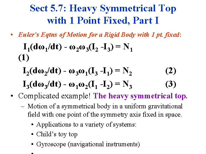
Sect 5. 7: Heavy Symmetrical Top with 1 Point Fixed, Part I • Euler’s Eqtns of Motion for a Rigid Body with 1 pt. fixed: I 1(dω1/dt) - ω2ω3(I 2 -I 3) = N 1 (1) I 2(dω2/dt) - ω3ω1(I 3 -I 1) = N 2 I 3(dω3/dt) - ω1ω2(I 1 -I 2) = N 3 (2) (3) • Complicated example! The heavy symmetrical top. – Motion of a symmetrical body in a uniform gravitational field with one point of the symmetry axis fixed in space. • Applications to a variety of systems: • Child’s toy top • Gyroscope (navigational instruments)

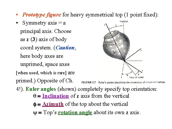
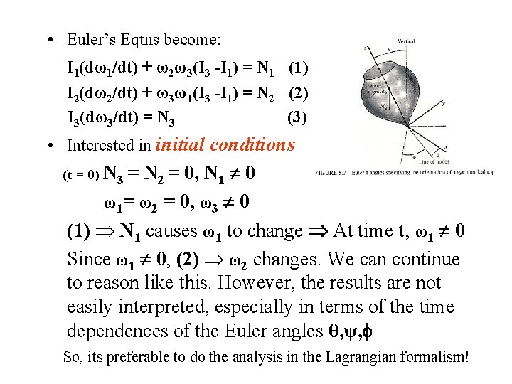
• Prototype figure for heavy symmetrical top (1 point fixed): • Symmetry axis = a principal axis. Choose as z (3) axis of body coord system. (Caution, here body axes are unprimed, space axes [when used, which is rare] are primed. ) Opposite of Ch. 4!). Euler angles (shown) completely specify top orientation: θ Inclination of z axis from the vertical Azimuth of the top about the vertical ψ Top’s rotation angle about its own z axis.

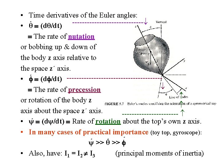
• Time derivatives of the Euler angles: • θ (dθ/dt) --------------- The rate of nutation or bobbing up & down of the body z axis relative to the space z´ axis. • (d /dt) ------------------- The rate of precession or rotation of the body z axis about the space z´ axis. ------------ • ψ (dψ/dt) Rate of rotation about the top’s own z axis. • In many cases of practical importance (toy top, gyroscope): ψ >> θ >> • Also, have: I 1 = I 2 I 3 (principal moments of inertia)

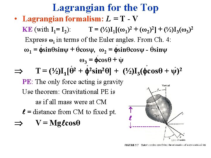
• Euler’s Eqtns become: I 1(dω1/dt) + ω2ω3(I 3 -I 1) = N 1 (1) I 2(dω2/dt) + ω3ω1(I 3 -I 1) = N 2 (2) I 3(dω3/dt) = N 3 (3) • Interested in initial conditions N 2 = 0, N 1 0 ω1= ω2 = 0, ω3 0 (1) N 1 causes ω1 to change At time t, ω1 0 Since ω1 0, (2) ω2 changes. We can continue to reason like this. However, the results are not easily interpreted, especially in terms of the time dependences of the Euler angles θ, ψ, (t = 0) N 3 = So, its preferable to do the analysis in the Lagrangian formalism!

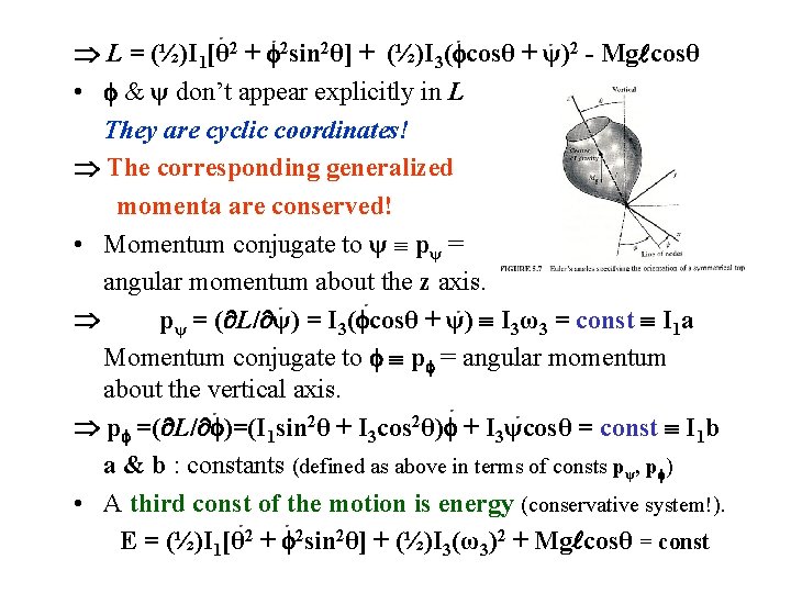
Lagrangian for the Top • Lagrangian formalism: L = T - V KE (with I 1= I 2): T = (½)I 1[(ω1)2 + (ω2)2] + (½)I 3(ω3)2 Express ωi in terms of the Euler angles. From Ch. 4: ω1 = sinθsinψ + θcosψ, ω2 = sinθcosψ - θsinψ ω3 = cosθ + ψ T = (½)I 1[θ 2 + 2 sin 2θ] + (½)I 3( cosθ + ψ)2 PE: The only force acting is gravity Use theorem: Gravitational PE is as if all mass were at CM _______ = distance from CM to fixed pt. V = Mg cosθ -------

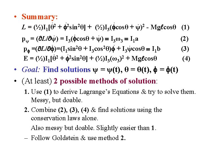
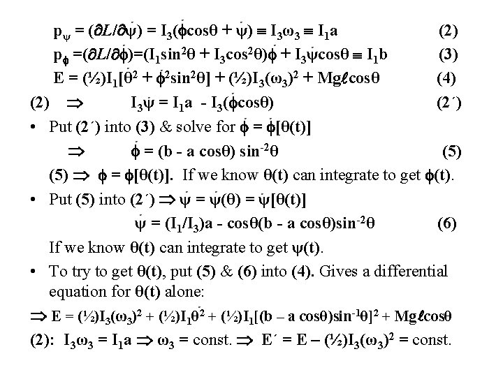
L = (½)I 1[θ 2 + 2 sin 2θ] + (½)I 3( cosθ + ψ)2 - Mg cosθ • & ψ don’t appear explicitly in L They are cyclic coordinates! The corresponding generalized momenta are conserved! • Momentum conjugate to ψ pψ = angular momentum about the z axis. pψ = ( L/ ψ) = I 3( cosθ + ψ) I 3ω3 = const I 1 a Momentum conjugate to p = angular momentum about the vertical axis. p =( L/ )=(I 1 sin 2θ + I 3 cos 2θ) + I 3ψcosθ = const I 1 b a & b : constants (defined as above in terms of consts pψ, p ) • A third const of the motion is energy (conservative system!). E = (½)I 1[θ 2 + 2 sin 2θ] + (½)I 3(ω3)2 + Mg cosθ = const

• Summary: L = (½)I 1[θ 2 + 2 sin 2θ] + (½)I 3( cosθ + ψ)2 - Mg cosθ (1) pψ = ( L/ ψ) = I 3( cosθ + ψ) I 3ω3 I 1 a p =( L/ )=(I 1 sin 2θ + I 3 cos 2θ) + I 3ψcosθ I 1 b E = (½)I 1[θ 2 + 2 sin 2θ] + (½)I 3(ω3)2 + Mg cosθ (2) (3) (4) • Goal: Find solutions ψ = ψ(t), θ = θ(t), = (t) • (At least) 2 possible methods of solution: 1. Use (1) to derive Lagrange’s Equations & try to solve them. Messy, but doable. 2. Combine (2), (3), (4) & find solutions using the conservation laws alone. Also messy but doable. Slightly easier than 1. – Follow Goldstein & use method 2.

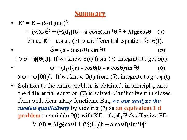
pψ = ( L/ ψ) = I 3( cosθ + ψ) I 3ω3 I 1 a (2) p =( L/ )=(I 1 sin 2θ + I 3 cos 2θ) + I 3ψcosθ I 1 b (3) E = (½)I 1[θ 2 + 2 sin 2θ] + (½)I 3(ω3)2 + Mg cosθ (4) (2) I 3ψ = I 1 a - I 3( cosθ) (2´) • Put (2´) into (3) & solve for = [θ(t)] = (b - a cosθ) sin-2θ (5) = [θ(t)]. If we know θ(t) can integrate to get (t). • Put (5) into (2´) ψ = ψ(θ) = ψ[θ(t)] ψ = (I 1/I 3)a - cosθ(b - a cosθ)sin-2θ (6) If we know θ(t) can integrate to get ψ(t). • To try to get θ(t), put (5) & (6) into (4). Gives a differential equation for θ(t) alone: E = (½)I 3(ω3)2 + (½)I 1θ 2 + (½)I 1[(b – a cosθ)sin-1θ]2 + Mg cosθ (2): I 3ω3 = I 1 a ω3 = const. E´ = E – (½)I 3(ω3)2 = const.

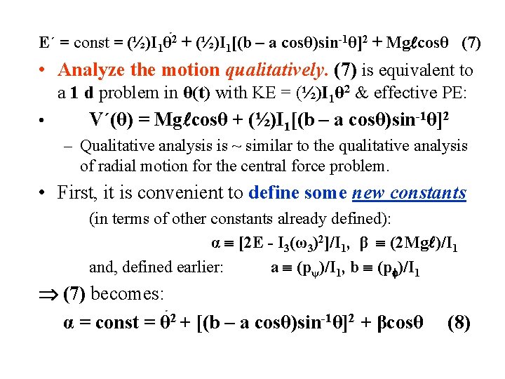
Summary • E´ = E – (½)I 3(ω3)2 = (½)I 1θ 2 + (½)I 1[(b – a cosθ)sin-1θ]2 + Mg cosθ (7) Since E´ = const, (7) is a differential equation for θ(t). • = (b - a cosθ) sin-2θ (5) = [θ(t)]. If we know θ(t) from (7), integrate to get (t). • ψ = (I 1/I 3)a - cosθ(b - a cosθ)sin-2θ (6) ψ = ψ[θ(t)]. If we know θ(t) from (7), integrate to get ψ(t). • Solution to the entire problem is obtained, in principle, once the differential equation (7) is solved. Can’t solve it in closed form with elementary functions. But, we can analyze the motion qualitatively by viewing (7) as an equivalent 1 d problem in variable θ(t) with KE = (½)I 1θ 2 & effective PE: V´(θ) = Mg cosθ + (½)I 1[(b – a cosθ)sin-1θ]2

E´ = const = (½)I 1θ 2 + (½)I 1[(b – a cosθ)sin-1θ]2 + Mg cosθ (7) • Analyze the motion qualitatively. (7) is equivalent to a 1 d problem in θ(t) with KE = (½)I 1θ 2 & effective PE: • V´(θ) = Mg cosθ + (½)I 1[(b – a cosθ)sin-1θ]2 – Qualitative analysis is ~ similar to the qualitative analysis of radial motion for the central force problem. • First, it is convenient to define some new constants (in terms of other constants already defined): α [2 E - I 3(ω3)2]/I 1, β (2 Mg )/I 1 and, defined earlier: a (pψ)/I 1, b (p )/I 1 (7) becomes: α = const = θ 2 + [(b – a cosθ)sin-1θ]2 + βcosθ (8)

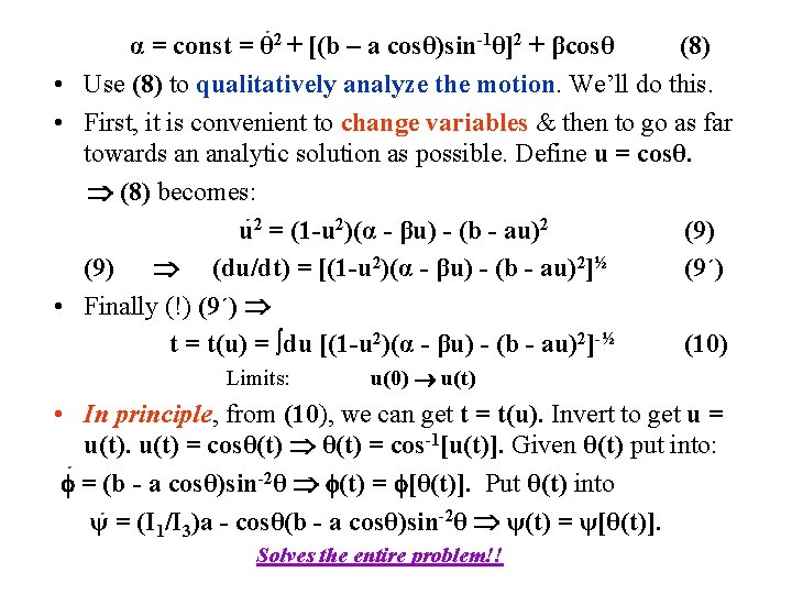
α = const = θ 2 + [(b – a cosθ)sin-1θ]2 + βcosθ (8) • Use (8) to qualitatively analyze the motion. We’ll do this. • First, it is convenient to change variables & then to go as far towards an analytic solution as possible. Define u = cosθ. (8) becomes: u 2 = (1 -u 2)(α - βu) - (b - au)2 (9) (du/dt) = [(1 -u 2)(α - βu) - (b - au)2]½ (9´) • Finally (!) (9´) t = t(u) = ∫du [(1 -u 2)(α - βu) - (b - au)2]-½ (10) Limits: u(0) u(t) • In principle, from (10), we can get t = t(u). Invert to get u = u(t) = cosθ(t) = cos-1[u(t)]. Given θ(t) put into: = (b - a cosθ)sin-2θ (t) = [θ(t)]. Put θ(t) into ψ = (I 1/I 3)a - cosθ(b - a cosθ)sin-2θ ψ(t) = ψ[θ(t)]. Solves the entire problem!!

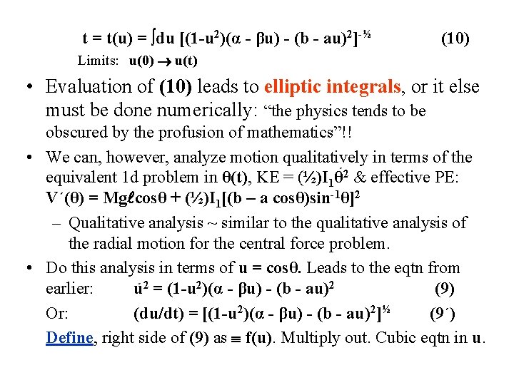
t = t(u) = ∫du [(1 -u 2)(α - βu) - (b - au)2]-½ (10) Limits: u(0) u(t) • Evaluation of (10) leads to elliptic integrals, or it else must be done numerically: “the physics tends to be obscured by the profusion of mathematics”!! • We can, however, analyze motion qualitatively in terms of the equivalent 1 d problem in θ(t), KE = (½)I 1θ 2 & effective PE: V´(θ) = Mg cosθ + (½)I 1[(b – a cosθ)sin-1θ]2 – Qualitative analysis ~ similar to the qualitative analysis of the radial motion for the central force problem. • Do this analysis in terms of u = cosθ. Leads to the eqtn from earlier: u 2 = (1 -u 2)(α - βu) - (b - au)2 (9) Or: (du/dt) = [(1 -u 2)(α - βu) - (b - au)2]½ (9´) Define, right side of (9) as f(u). Multiply out. Cubic eqtn in u.

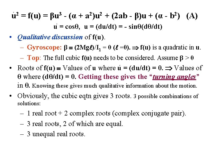
u 2 = f(u) = βu 3 - (α + a 2)u 2 + (2 ab - β)u + (α - b 2) (A) u = cosθ, u = (du/dt) = - sinθ(dθ/dt) • Qualitative discussion of f(u). – Gyroscope: β (2 Mg )/I 1 = 0 ( =0). f(u) is a quadratic in u. – Top: The full cubic f(u) needs to be considered. Assume β > 0 • Roots of f(u) Values of u where u = (du/dt) = 0. Values of θ where (dθ/dt) = 0. Getting these gives the “turning angles” in θ. Knowing these gives much qualitative information about the motion. • Obviously, the cubic eqtn gives 3 roots. 3 possible combinations of solutions: – 1 real root + 2 complex roots (complex conjugate pair). – 3 real roots, 2 of which are equal. – 3 unequal real roots.

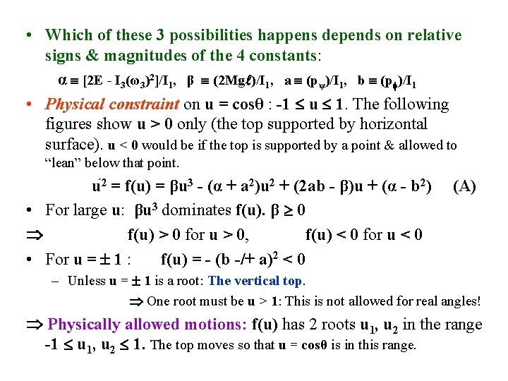
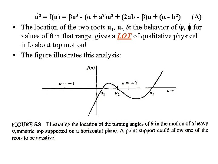
• Which of these 3 possibilities happens depends on relative signs & magnitudes of the 4 constants: α [2 E - I 3(ω3)2]/I 1, β (2 Mg )/I 1, a (pψ)/I 1, b (p )/I 1 • Physical constraint on u = cosθ : -1 u 1. The following figures show u > 0 only (the top supported by horizontal surface). u < 0 would be if the top is supported by a point & allowed to “lean” below that point. u 2 = f(u) = βu 3 - (α + a 2)u 2 + (2 ab - β)u + (α - b 2) • For large u: βu 3 dominates f(u). β 0 f(u) > 0 for u > 0, f(u) < 0 for u < 0 • For u = 1 : f(u) = - (b -/+ a)2 < 0 (A) – Unless u = 1 is a root: The vertical top. One root must be u > 1: This is not allowed for real angles! Physically allowed motions: f(u) has 2 roots u 1, u 2 in the range -1 u 1, u 2 1. The top moves so that u = cosθ is in this range.

u 2 = f(u) = βu 3 - (α + a 2)u 2 + (2 ab - β)u + (α - b 2) (A) • The location of the two roots u 1, u 2 & the behavior of ψ, for values of θ in that range, gives a LOT of qualitative physical info about top motion! • The figure illustrates this analysis:

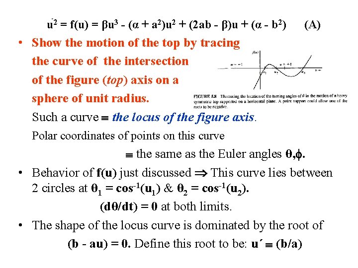
u 2 = f(u) = βu 3 - (α + a 2)u 2 + (2 ab - β)u + (α - b 2) (A) • Show the motion of the top by tracing the curve of the intersection of the figure (top) axis on a sphere of unit radius. Such a curve the locus of the figure axis. Polar coordinates of points on this curve the same as the Euler angles θ, . • Behavior of f(u) just discussed This curve lies between 2 circles at θ 1 = cos-1(u 1) & θ 2 = cos-1(u 2). (dθ/dt) = 0 at both limits. • The shape of the locus curve is dominated by the root of (b - au) = 0. Define this root to be: u´ (b/a)

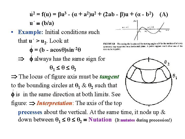
u 2 = f(u) = βu 3 - (α + a 2)u 2 + (2 ab - β)u + (α - b 2) (A) u´ (b/a) • Example: Initial conditions such that u´ > u 2. Look at = (b - acosθ)sin-2θ always has the same sign for θ 1 θ θ 2 The locus of figure axis must be tangent to the bounding circles at θ 1 & θ 2 such that is in the same direction at both limits. See figure: Interpretation: The axis of the top precesses about the vertical. At the same time, it nods up & down between θ 1 θ θ 2 Nutation (It nutates during precession!)

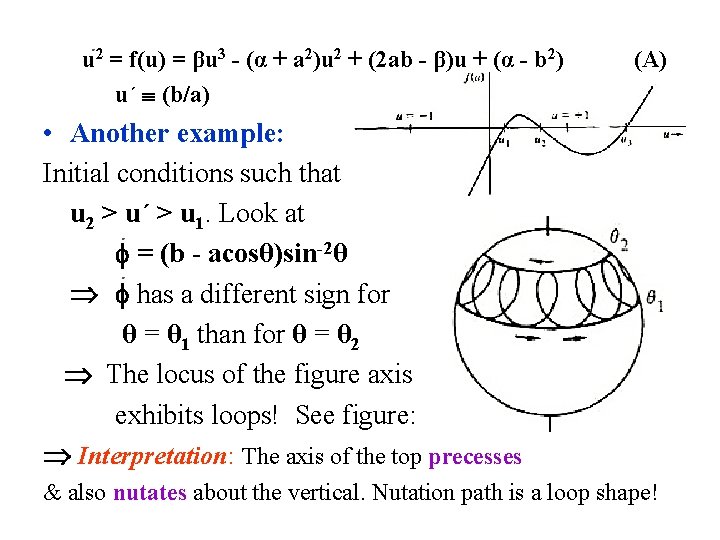
u 2 = f(u) = βu 3 - (α + a 2)u 2 + (2 ab - β)u + (α - b 2) u´ (b/a) (A) • Another example: Initial conditions such that u 2 > u´ > u 1. Look at = (b - acosθ)sin-2θ has a different sign for θ = θ 1 than for θ = θ 2 The locus of the figure axis exhibits loops! See figure: Interpretation: The axis of the top precesses & also nutates about the vertical. Nutation path is a loop shape!

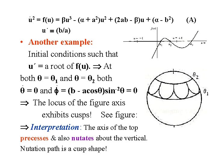
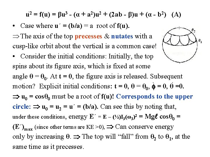
u 2 = f(u) = βu 3 - (α + a 2)u 2 + (2 ab - β)u + (α - b 2) u´ (b/a) • Another example: Initial conditions such that u´ = a root of f(u). At both θ = θ 1 and θ = θ 2 both θ = 0 and = (b - acosθ)sin-2θ = 0 The locus of the figure axis exhibits cusps! See figure: Interpretation: The axis of the top precesses & also nutates about the vertical. Nutation path is a cusp shape! (A)

u 2 = f(u) = βu 3 - (α + a 2)u 2 + (2 ab - β)u + (α - b 2) (A) • Case where u´ = (b/a) = a root of f(u). The axis of the top precesses & nutates with a cusp-like orbit about the vertical is a common case! • Consider the initial conditions: Initially, the top spins about its figure axis, which is fixed at some angle θ = θ 0. At t = 0, the figure axis is released. Subsequent motion? Explicit initial conditions: t = 0, θ = θ 0, = 0, θ =0. u 0 = cosθ 0 must be a root of f(u)! Corresponds to the upper circle: u 0 = u 2 = u´ = (b/a). Can see this by noting that, under these conditions, energy E´ = E – (½)I 3(ω3)2 = Mg cosθ 0 = (E´)max (since other terms are KE >0), Can conserve energy only by increasing θ. The top will “fall” from θ 2 to θ 1, at the same time as it precesses.