Sec 18 1 NEWTONS DIVIDEDDIFFERENCE INTERPOLATING POLYNOMIALS Sec

Sec: 18. 1 NEWTON’S DIVIDEDDIFFERENCE INTERPOLATING POLYNOMIALS

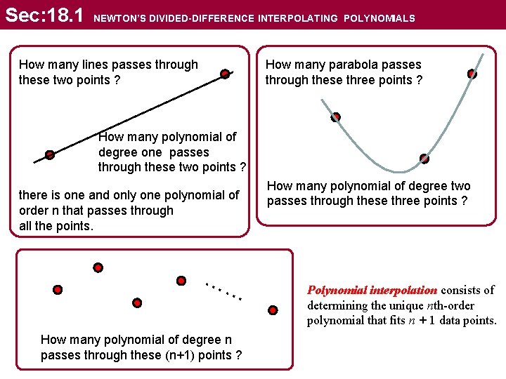
Sec: 18. 1 NEWTON’S DIVIDED-DIFFERENCE INTERPOLATING POLYNOMIALS How many lines passes through these two points ? How many parabola passes through these three points ? How many polynomial of degree one passes through these two points ? there is one and only one polynomial of order n that passes through all the points. …… How many polynomial of degree n passes through these (n+1) points ? How many polynomial of degree two passes through these three points ? Polynomial interpolation consists of determining the unique nth-order polynomial that fits n + 1 data points.

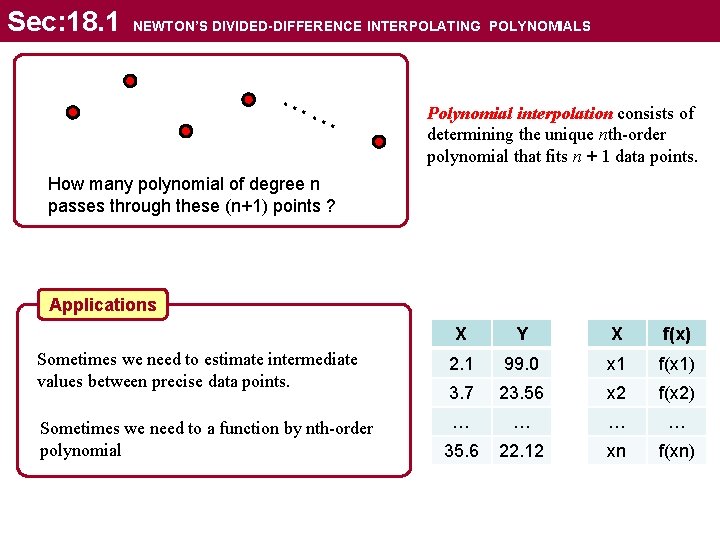
Sec: 18. 1 NEWTON’S DIVIDED-DIFFERENCE INTERPOLATING POLYNOMIALS …… Polynomial interpolation consists of determining the unique nth-order polynomial that fits n + 1 data points. How many polynomial of degree n passes through these (n+1) points ? Applications X Y X f(x) Sometimes we need to estimate intermediate values between precise data points. 2. 1 99. 0 x 1 f(x 1) 3. 7 23. 56 x 2 f(x 2) Sometimes we need to a function by nth-order polynomial … … 35. 6 22. 12 xn f(xn)

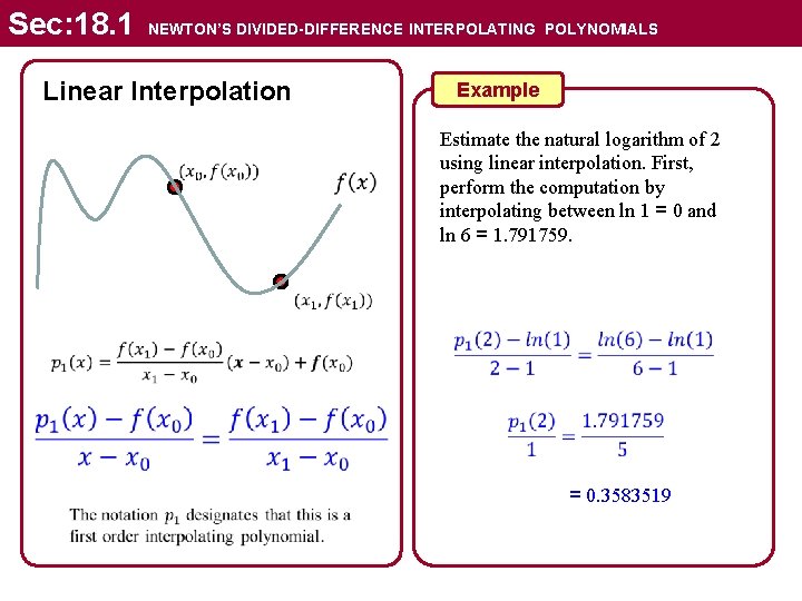
Sec: 18. 1 NEWTON’S DIVIDED-DIFFERENCE INTERPOLATING POLYNOMIALS Linear Interpolation Example Estimate the natural logarithm of 2 using linear interpolation. First, perform the computation by interpolating between ln 1 = 0 and ln 6 = 1. 791759. = 0. 3583519

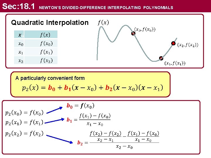
Sec: 18. 1 NEWTON’S DIVIDED-DIFFERENCE INTERPOLATING POLYNOMIALS Quadratic Interpolation A particularly convenient form

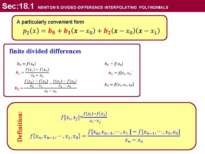
Sec: 18. 1 NEWTON’S DIVIDED-DIFFERENCE INTERPOLATING POLYNOMIALS A particularly convenient form finite divided differences Definition:

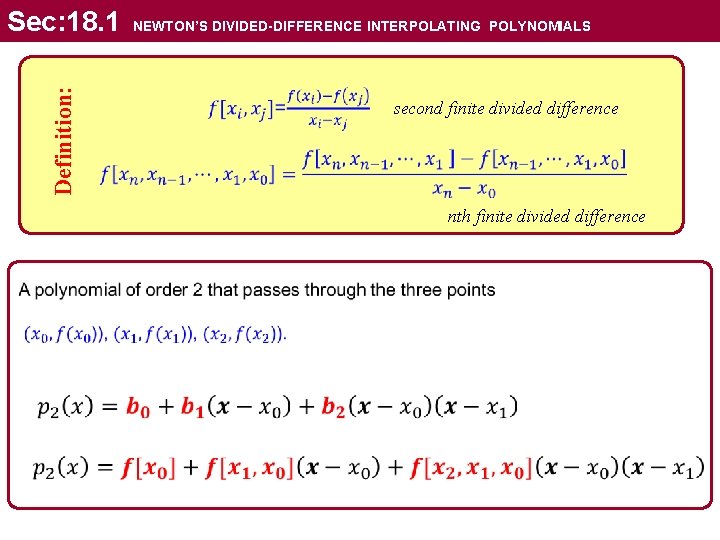
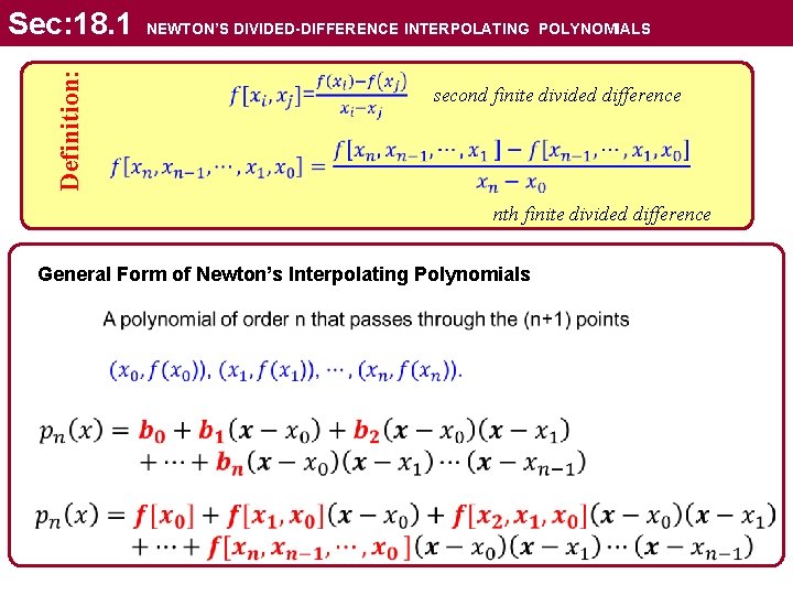
Definition: Sec: 18. 1 NEWTON’S DIVIDED-DIFFERENCE INTERPOLATING POLYNOMIALS second finite divided difference nth finite divided difference

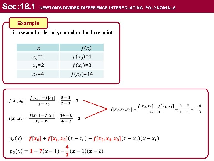
Sec: 18. 1 NEWTON’S DIVIDED-DIFFERENCE INTERPOLATING POLYNOMIALS Example Fit a second-order polynomial to the three points

Definition: Sec: 18. 1 NEWTON’S DIVIDED-DIFFERENCE INTERPOLATING POLYNOMIALS second finite divided difference nth finite divided difference General Form of Newton’s Interpolating Polynomials

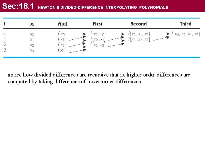
Sec: 18. 1 NEWTON’S DIVIDED-DIFFERENCE INTERPOLATING POLYNOMIALS notice how divided differences are recursive that is, higher-order differences are computed by taking differences of lower-order differences.

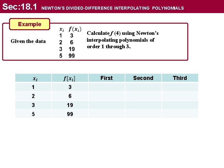
Sec: 18. 1 NEWTON’S DIVIDED-DIFFERENCE INTERPOLATING POLYNOMIALS Example Calculate f (4) using Newton’s interpolating polynomials of order 1 through 3. Given the data First 1 3 2 6 3 19 5 99 Second Third

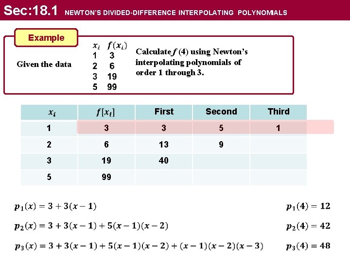
Sec: 18. 1 NEWTON’S DIVIDED-DIFFERENCE INTERPOLATING POLYNOMIALS Example Calculate f (4) using Newton’s interpolating polynomials of order 1 through 3. Given the data First Second Third 1 1 3 3 5 2 6 13 9 3 19 40 5 99

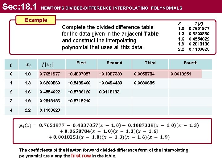
Sec: 18. 1 NEWTON’S DIVIDED-DIFFERENCE INTERPOLATING POLYNOMIALS Example Complete the divided difference table for the data given in the adjacent Table and construct the interpolating polynomial that uses all this data. Second Third − 0. 4837057 − 0. 1087339 0. 0658784 0. 6200860 − 0. 5489460 − 0. 0494433 0. 0680685 1. 6 0. 4554022 − 0. 5786120 0. 0118183 3 1. 9 0. 2818186 − 0. 5715210 4 2. 2 0. 1103623 0 1. 0 0. 7651977 1 1. 3 2 First x 1. 0 1. 3 1. 6 1. 9 2. 2 f (x) 0. 7651977 0. 6200860 0. 4554022 0. 2818186 0. 1103623 Fourth 0. 0018251 The coefficients of the Newton forward divided-difference form of the interpolating polynomial are along the first row in the table.

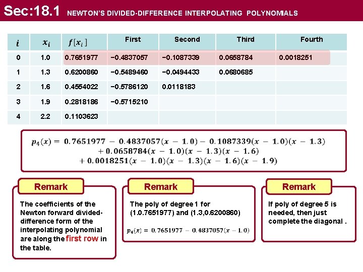
Sec: 18. 1 NEWTON’S DIVIDED-DIFFERENCE INTERPOLATING POLYNOMIALS Second Third − 0. 4837057 − 0. 1087339 0. 0658784 0. 6200860 − 0. 5489460 − 0. 0494433 0. 0680685 1. 6 0. 4554022 − 0. 5786120 0. 0118183 3 1. 9 0. 2818186 − 0. 5715210 4 2. 2 0. 1103623 0 1. 0 0. 7651977 1 1. 3 2 First Fourth 0. 0018251 Remark The coefficients of the Newton forward divideddifference form of the interpolating polynomial are along the first row in the table. Remark The poly of degree 1 for (1. 0. 7651977) and (1. 3, 0. 6200860) Remark If poly of degree 5 is needed, then just complete the diagonal.

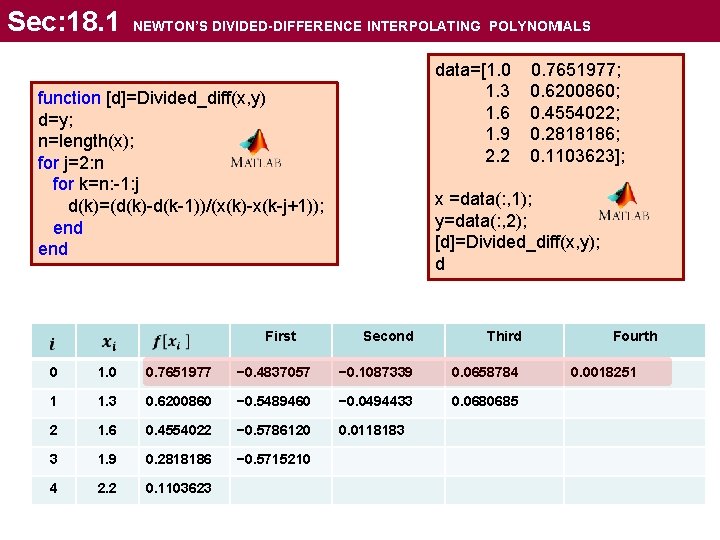
Sec: 18. 1 NEWTON’S DIVIDED-DIFFERENCE INTERPOLATING POLYNOMIALS data=[1. 0 0. 7651977; 1. 3 0. 6200860; 1. 6 0. 4554022; 1. 9 0. 2818186; 2. 2 0. 1103623]; x =data(: , 1); y=data(: , 2); [d]=Divided_diff(x, y); d function [d]=Divided_diff(x, y) d=y; n=length(x); for j=2: n for k=n: -1: j d(k)=(d(k)-d(k-1))/(x(k)-x(k-j+1)); end Second Third − 0. 4837057 − 0. 1087339 0. 0658784 0. 6200860 − 0. 5489460 − 0. 0494433 0. 0680685 1. 6 0. 4554022 − 0. 5786120 0. 0118183 3 1. 9 0. 2818186 − 0. 5715210 4 2. 2 0. 1103623 0 1. 0 0. 7651977 1 1. 3 2 First Fourth 0. 0018251

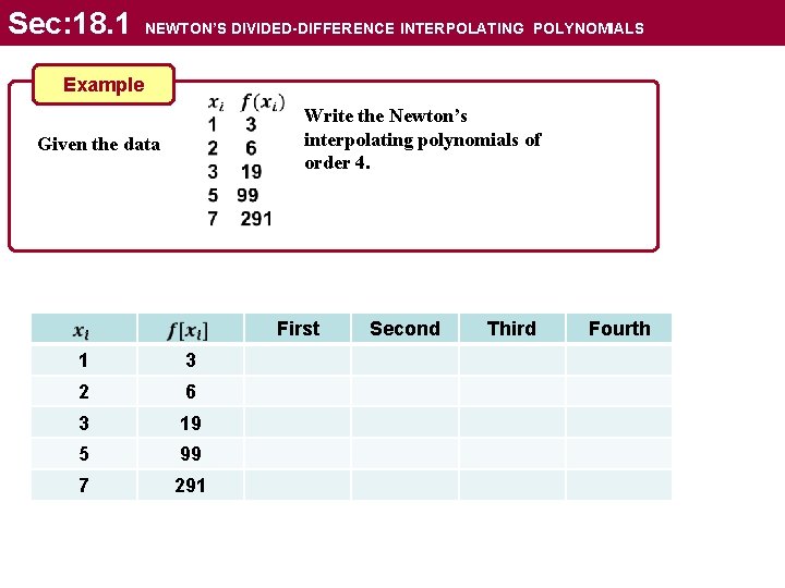
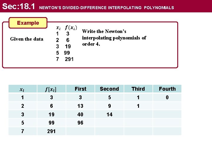
Sec: 18. 1 NEWTON’S DIVIDED-DIFFERENCE INTERPOLATING POLYNOMIALS Example Given the data Write the Newton’s interpolating polynomials of order 4. First 1 3 2 6 3 19 5 99 7 291 Second Third Fourth

Sec: 18. 1 NEWTON’S DIVIDED-DIFFERENCE INTERPOLATING POLYNOMIALS Example Write the Newton’s interpolating polynomials of order 4. Given the data First Second Third Fourth 0 1 3 3 5 1 2 6 13 9 1 3 19 40 14 5 99 96 7 291

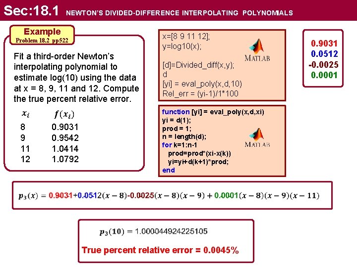
Sec: 18. 1 NEWTON’S DIVIDED-DIFFERENCE INTERPOLATING POLYNOMIALS Example Problem 18. 2 pp 522 Fit a third-order Newton’s interpolating polynomial to estimate log(10) using the data at x = 8, 9, 11 and 12. Compute the true percent relative error. 8 9 11 12 x=[8 9 11 12]; y=log 10(x); [d]=Divided_diff(x, y); d [yi] = eval_poly(x, d, 10) Rel_err = (yi-1)/1*100 function [yi] = eval_poly(x, d, xi) yi = d(1); prod = 1; n = length(d); for k=1: n-1 prod=prod*(xi-x(k)) yi=yi+d(k+1)*prod; end 0. 9031 0. 9542 1. 0414 1. 0792 True percent relative error = 0. 0045% 0. 9031 0. 0512 -0. 0025 0. 0001

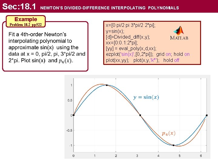
Sec: 18. 1 NEWTON’S DIVIDED-DIFFERENCE INTERPOLATING POLYNOMIALS Example Problem 18. 2 pp 522 x=[0 pi/2 pi 3*pi/2 2*pi]; y=sin(x); [d]=Divided_diff(x, y); xx=[0: 0. 1: 2*pi]; [yy] = eval_poly(x, d, xx); ezplot('sin(x)', [0, 2*pi]); grid on; hold on plot(xx, yy); plot(x, y, 'k*'); hold off

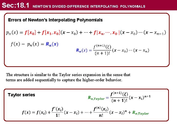
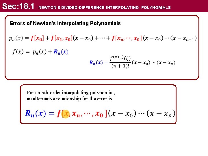
Sec: 18. 1 NEWTON’S DIVIDED-DIFFERENCE INTERPOLATING POLYNOMIALS Errors of Newton’s Interpolating Polynomials The structure is similar to the Taylor series expansion in the sense that terms are added sequentially to capture the higher-order behavior. Taylor series

Sec: 18. 1 NEWTON’S DIVIDED-DIFFERENCE INTERPOLATING POLYNOMIALS Errors of Newton’s Interpolating Polynomials For an nth-order interpolating polynomial, an alternative relationship for the error is

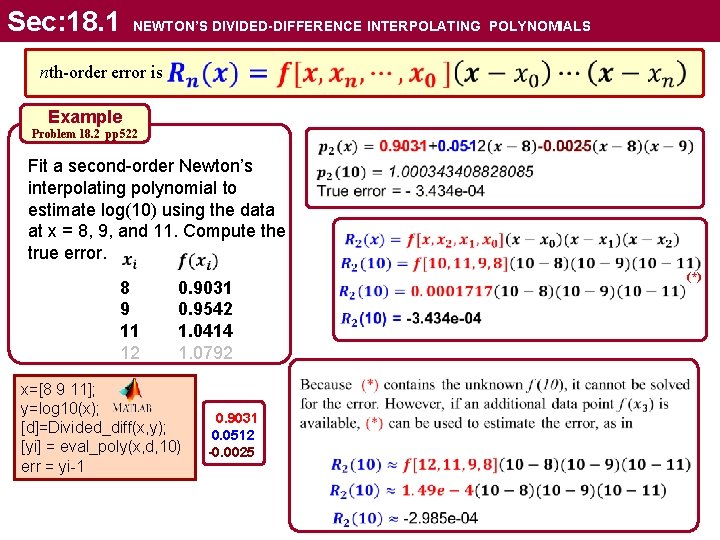
Sec: 18. 1 NEWTON’S DIVIDED-DIFFERENCE INTERPOLATING POLYNOMIALS nth-order error is Example Problem 18. 2 pp 522 Fit a second-order Newton’s interpolating polynomial to estimate log(10) using the data at x = 8, 9, and 11. Compute the true error. 8 0. 9031 9 0. 9542 11 1. 0414 12 1. 0792 x=[8 9 11]; y=log 10(x); 0. 9031 [d]=Divided_diff(x, y); 0. 0512 [yi] = eval_poly(x, d, 10) -0. 0025 err = yi-1 (*)

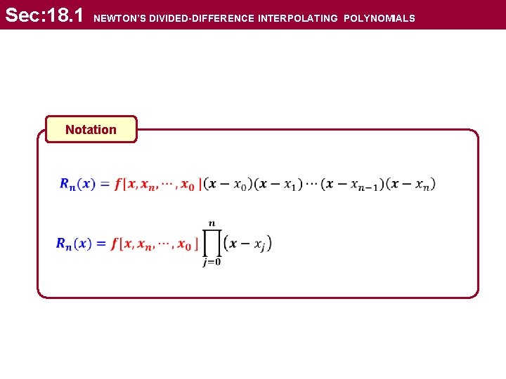
Sec: 18. 1 NEWTON’S DIVIDED-DIFFERENCE INTERPOLATING POLYNOMIALS Notation