Sec 18 2 LAGRANGE INTERPOLATING POLYNOMIALS Sec 18
- Slides: 11

Sec: 18. 2 LAGRANGE INTERPOLATING POLYNOMIALS

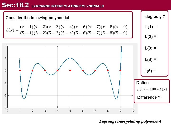
Sec: 18. 2 LAGRANGE INTERPOLATING POLYNOMIALS Consider the following polynomial deg poly ? L(1) = L(2) = L(9) = L(8) = L(5) = Define: Difference ? Lagrange interpolating polynomial

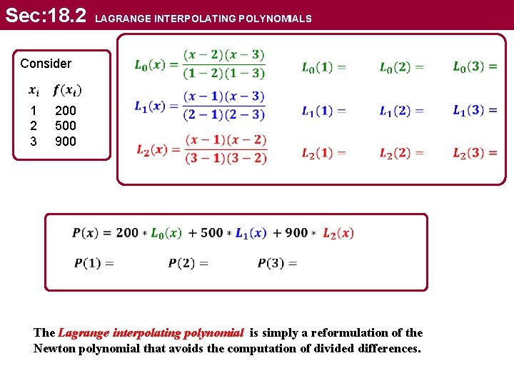
Sec: 18. 2 Consider LAGRANGE INTERPOLATING POLYNOMIALS 1 200 2 500 3 900 The Lagrange interpolating polynomial is simply a reformulation of the Newton polynomial that avoids the computation of divided differences.

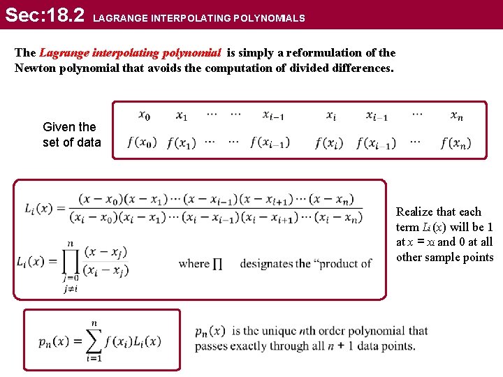
Sec: 18. 2 LAGRANGE INTERPOLATING POLYNOMIALS The Lagrange interpolating polynomial is simply a reformulation of the Newton polynomial that avoids the computation of divided differences. Given the set of data Realize that each term Li (x) will be 1 at x = xi and 0 at all other sample points

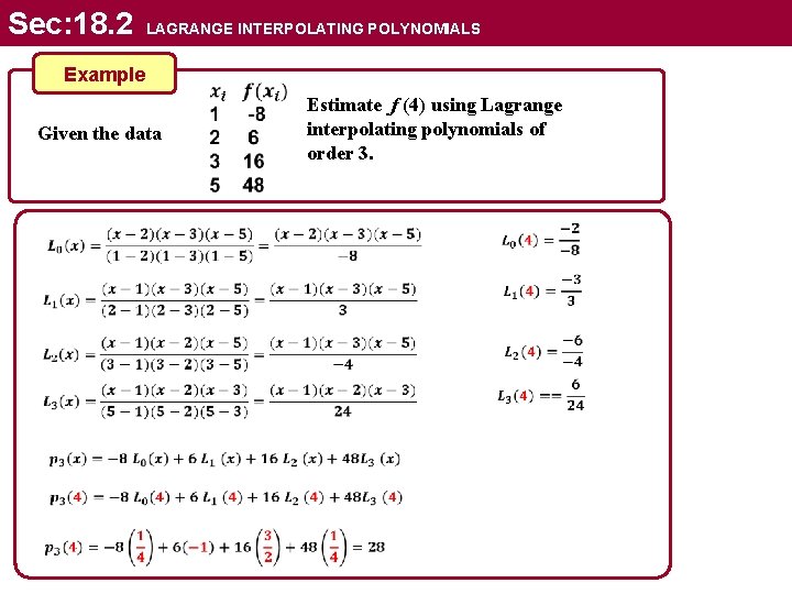
Sec: 18. 2 LAGRANGE INTERPOLATING POLYNOMIALS Example Given the data Estimate f (4) using Lagrange interpolating polynomials of order 3.

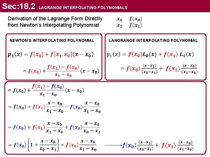
Sec: 18. 2 LAGRANGE INTERPOLATING POLYNOMIALS Derivation of the Lagrange Form Directly from Newton’s Interpolating Polynomial NEWTON’S INTERPOLATING POLYNOMIAL LANGRANGE INTERPOLATING POLYNOMIAL

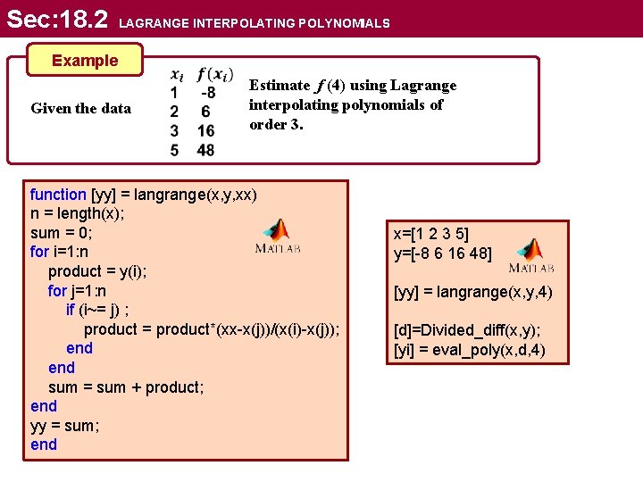
Sec: 18. 2 LAGRANGE INTERPOLATING POLYNOMIALS Example Given the data Estimate f (4) using Lagrange interpolating polynomials of order 3. function [yy] = langrange(x, y, xx) n = length(x); sum = 0; for i=1: n product = y(i); for j=1: n if (i~= j) ; product = product*(xx-x(j))/(x(i)-x(j)); end sum = sum + product; end yy = sum; end x=[1 2 3 5] y=[-8 6 16 48] [yy] = langrange(x, y, 4) [d]=Divided_diff(x, y); [yi] = eval_poly(x, d, 4)

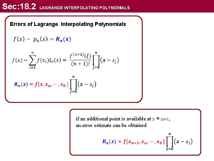
Sec: 18. 2 LAGRANGE INTERPOLATING POLYNOMIALS Errors of Lagrange Interpolating Polynomials if an additional point is available at x = xn+1, an error estimate can be obtained

Sec: 18. 2 LAGRANGE INTERPOLATING POLYNOMIALS In summary, for cases where the order of the polynomial is unknown, the Newton method has advantages because of the insight it provides into the behavior of the different order formulas. In addition, the error estimate can usually be integrated easily into the Newton computation because the estimate employs a finite difference. Thus, for exploratory computations, Newton’s method is often preferable. When only one interpolation is to be performed, the Lagrange and Newton formulations require comparable computational effort. However, the Lagrange version is somewhat easier to program. Because it does not require computation and storage of divided differences, the Lagrange form is often used when the order of the polynomial is known a priori.

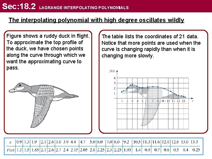
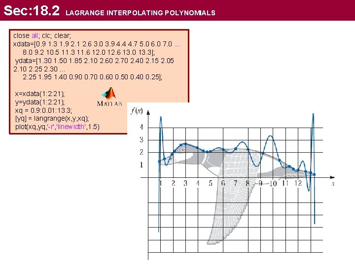
Sec: 18. 2 LAGRANGE INTERPOLATING POLYNOMIALS The interpolating polynomial with high degree oscillates wildly Figure shows a ruddy duck in flight. To approximate the top profile of the duck, we have chosen points along the curve through which we want the approximating curve to pass. The table lists the coordinates of 21 data. Notice that more points are used when the curve is changing rapidly than when it is changing more slowly.

Sec: 18. 2 LAGRANGE INTERPOLATING POLYNOMIALS close all; clc; clear; xdata=[0. 9 1. 3 1. 9 2. 1 2. 6 3. 0 3. 9 4. 4 4. 7 5. 0 6. 0 7. 0. . . 8. 0 9. 2 10. 5 11. 3 11. 6 12. 0 12. 6 13. 0 13. 3]; ydata=[1. 30 1. 50 1. 85 2. 10 2. 60 2. 70 2. 40 2. 15 2. 05 2. 10 2. 25 2. 30. . . 2. 25 1. 95 1. 40 0. 90 0. 70 0. 60 0. 50 0. 40 0. 25]; x=xdata(1: 2: 21); y=ydata(1: 2: 21); xq = 0. 9: 0. 01: 13. 3; [yq] = langrange(x, y, xq); plot(xq, yq, '-r', 'linewidth', 1. 5)