Scalar Analysis in Synoptic Meteorology ATMS 370 Definition

Scalar Analysis in Synoptic Meteorology ATMS 370

Definition • Scalar Analysis is the analysis of a quantity that has magnitude only • Examples: temperature and pressure. • Consists of drawing isopleths: line of constant values. Topographic maps are good examples.

Examples of Meteorological Isopleths • isobar: pressure • isohyet: precipitation • isopycnic: density • isotach: wind speed • isogon: wind direction • isotherm: temperature • isentrope: potential temperature • isallobar: pressure change isallobars

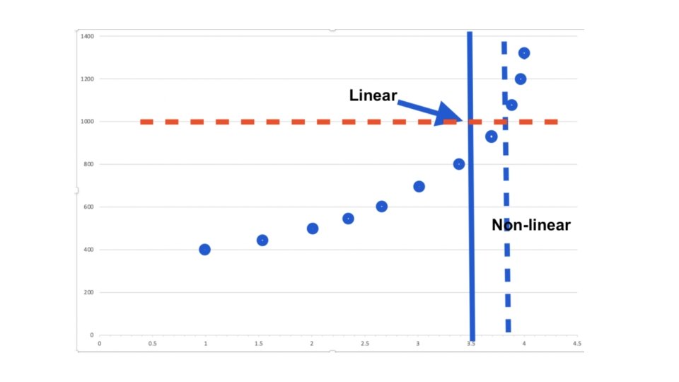
• Being with plotted map with some parameter at selected observation points. • Decide on contours and values. • Then interpolate between points as one draws continuous lines. 1200 800 1000 800 1400 1200 900

Linear interpolation is acceptable as first approximation, but non-linear variations should be taken into account if possible linear 400 500 Non-linear 700 1300

Both human and machine-based interpolation is possible: humans often do a very good job at it, even capturing non-linear effects • Human’s can gain understanding through manual analysis • That is one reason you will do so in class. • There is an intimate connection between our hands and brains • And a great deal of learning in making the subtle decisions about where to put isopleths.

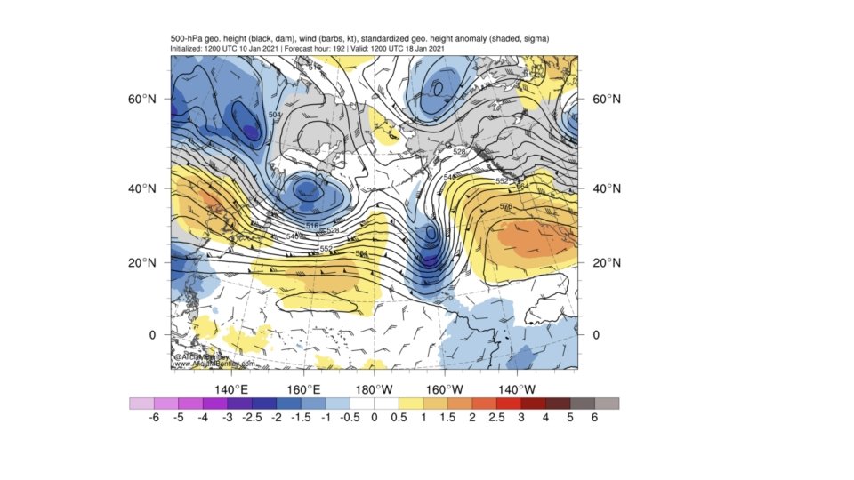
500 h. Pa: The first level you will analyze • Will analyze 500 h. Pa geopotential heights. Noting ridges, troughs, closed lows, closed highs. • Important level: about half the mass of atmosphere is above and below. ~5500 meters, 18, 000 ft. • 60 -m contour interval is standard • Centered around 5400 m. e. g. , 5280, 5340, 5400, 5460, 5520 meters • Labeled in decameter (dm)—hundreds of meters (e. g. , 540, 546)

Typical 500 h. Pa wave pattern Weaker gradient Tighter gradient

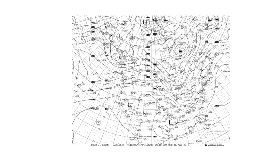
Important tip: You are doing a synoptic(larger scale) analysis. Keep lines smooth!

Where data is sparse, choose simple, regular spacing

NOT THIS

500 h. Pa analysis tips • Observations are not perfectly accurate, typically 500 h. Pa heights have errors of ~10 -15 meters. Thus, you have some flexibility. • Flow is very close to geostrophic at 500 h. Pa so: • Winds should be ~parallel to height lines • Wind speeds should be scaling with height gradient (winds stronger with greater gradients) • Thus, winds give you a lot of information about height lines

Sometimes there are discrepancies with geostrophy at 500 h. Pa • In tight troughs or ridges where the gradient wind balance is better than geostrophic • supergeostrophic winds in ridges • subgeostrphic winds in troughs. • More later in class! • Where there are observation errors • Due to subsynoptic features we are not analyzing (e. g. , thunderstorms)

Upper-Level Station Model (radiosonde) At 500 h. Pa, height (hhh) is In decameters. (553 is 5530 meter) Circle is shaded if dew point depression is five or less

* Indicates satellite based obs

Rectangle indicates aircraft-based observations