Sample Exercises Excel 2007 MULTIPLE CHOICE 1 A

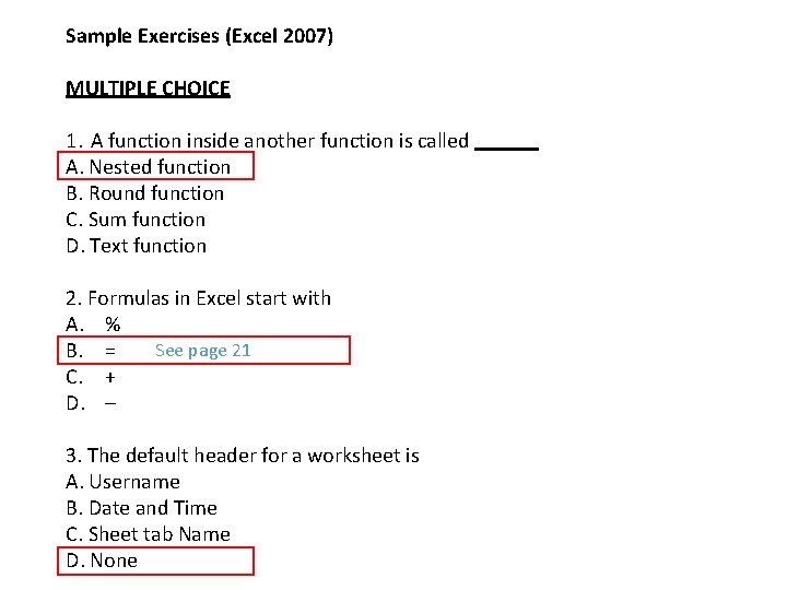
Sample Exercises (Excel 2007) MULTIPLE CHOICE 1. A function inside another function is called A. Nested function B. Round function C. Sum function D. Text function 2. Formulas in Excel start with A. % See page 21 B. = C. + D. – 3. The default header for a worksheet is A. Username B. Date and Time C. Sheet tab Name D. None

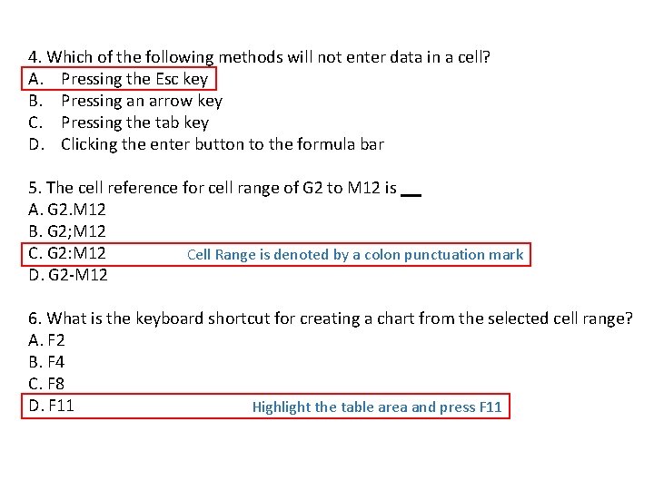
4. Which of the following methods will not enter data in a cell? A. Pressing the Esc key B. Pressing an arrow key C. Pressing the tab key D. Clicking the enter button to the formula bar 5. The cell reference for cell range of G 2 to M 12 is A. G 2. M 12 B. G 2; M 12 C. G 2: M 12 Cell Range is denoted by a colon punctuation mark D. G 2 -M 12 6. What is the keyboard shortcut for creating a chart from the selected cell range? A. F 2 B. F 4 C. F 8 D. F 11 Highlight the table area and press F 11

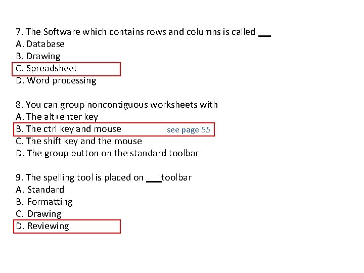
7. The Software which contains rows and columns is called A. Database B. Drawing C. Spreadsheet D. Word processing 8. You can group noncontiguous worksheets with A. The alt+enter key B. The ctrl key and mouse see page 55 C. The shift key and the mouse D. The group button on the standard toolbar 9. The spelling tool is placed on A. Standard B. Formatting C. Drawing D. Reviewing toolbar

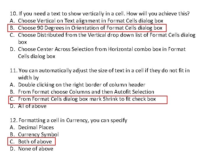
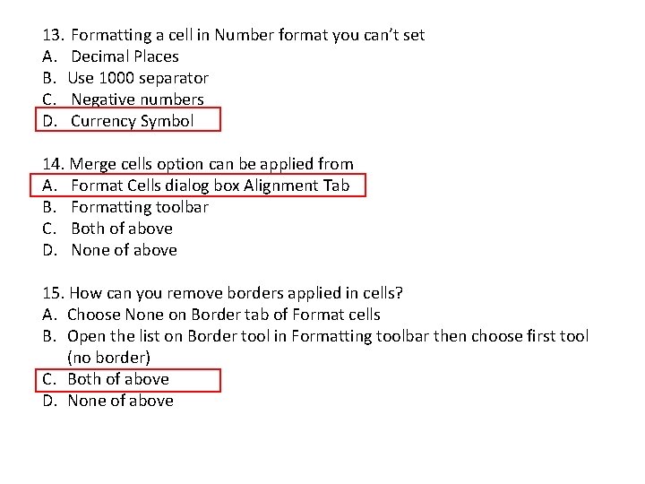
10. If you need a text to show vertically in a cell. How will you achieve this? A. Choose Vertical on Text alignment in Format Cells dialog box B. Choose 90 Degrees in Orientation of Format Cells dialog box C. Choose Distributed from the Vertical drop down list of Format Cells dialog box D. Choose Center Across Selection from Horizontal combo box in Format Cells dialog box 11. You can automatically adjust the size of text in a cell if they do not fit in width by A. Double clicking on the right border of column header B. From Format choose Columns and then Autofit Selection C. From Format Cells dialog box mark Shrink to fit check box D. All of above 12. Formatting a cell in Currency, you can specify A. Decimal Places B. Currency Symbol C. Both of above D. None of above

13. Formatting a cell in Number format you can’t set A. Decimal Places B. Use 1000 separator C. Negative numbers D. Currency Symbol 14. Merge cells option can be applied from A. Format Cells dialog box Alignment Tab B. Formatting toolbar C. Both of above D. None of above 15. How can you remove borders applied in cells? A. Choose None on Border tab of Format cells B. Open the list on Border tool in Formatting toolbar then choose first tool (no border) C. Both of above D. None of above

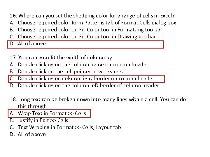
16. Where can you set the shedding color for a range of cells in Excel? A. Choose required color form Patterns tab of Format Cells dialog box B. Choose required color on Fill Color tool in Formatting toolbar C. Choose required color on Fill Color tool in Drawing toolbar D. All of above 17. You can auto fit the width of column by A. Double clicking on the column name on column header B. Double click on the cell pointer in worksheet C. Double clicking on column right border on column header D. Double clicking on the column left border of column header 18. Long text can be broken down into many lines within a cell. You can do this through A. Wrap Text in Format >> Cells B. Justify in Edit >> Cells C. Text Wraping in Format >> Cells, Layout tab D. All of above

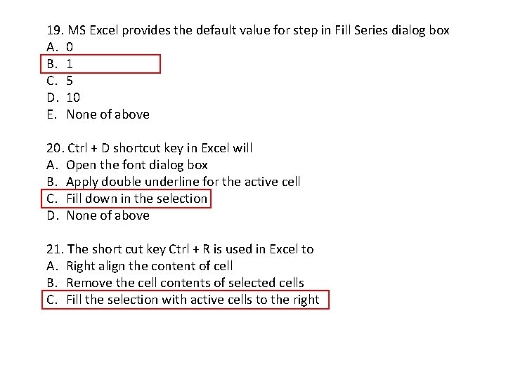
19. MS Excel provides the default value for step in Fill Series dialog box A. 0 B. 1 C. 5 D. 10 E. None of above 20. Ctrl + D shortcut key in Excel will A. Open the font dialog box B. Apply double underline for the active cell C. Fill down in the selection D. None of above 21. The short cut key Ctrl + R is used in Excel to A. Right align the content of cell B. Remove the cell contents of selected cells C. Fill the selection with active cells to the right

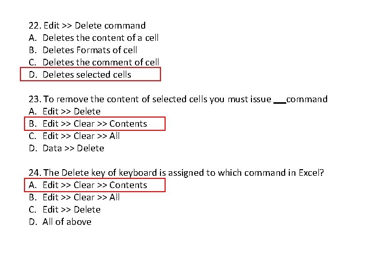
22. Edit >> Delete command A. Deletes the content of a cell B. Deletes Formats of cell C. Deletes the comment of cell D. Deletes selected cells 23. To remove the content of selected cells you must issue A. Edit >> Delete B. Edit >> Clear >> Contents C. Edit >> Clear >> All D. Data >> Delete command 24. The Delete key of keyboard is assigned to which command in Excel? A. Edit >> Clear >> Contents B. Edit >> Clear >> All C. Edit >> Delete D. All of above

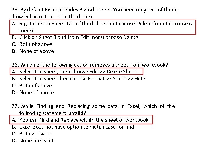
25. By default Excel provides 3 worksheets. You need only two of them, how will you delete third one? A. Right click on Sheet Tab of third sheet and choose Delete from the context menu B. Click on Sheet 3 and from Edit menu choose Delete C. Both of above D. None of above 26. Which of the following action removes a sheet from workbook? A. Select the sheet, then choose Edit >> Delete Sheet B. Select the sheet then choose Format >> Sheet >> Hide C. Both of above D. None of above 27. While Finding and Replacing some data in Excel, which of the following statement is valid? A. You can Find and Replace within the sheet or workbook B. Excel does not have option to match case for find C. Both are valid D. None are valid

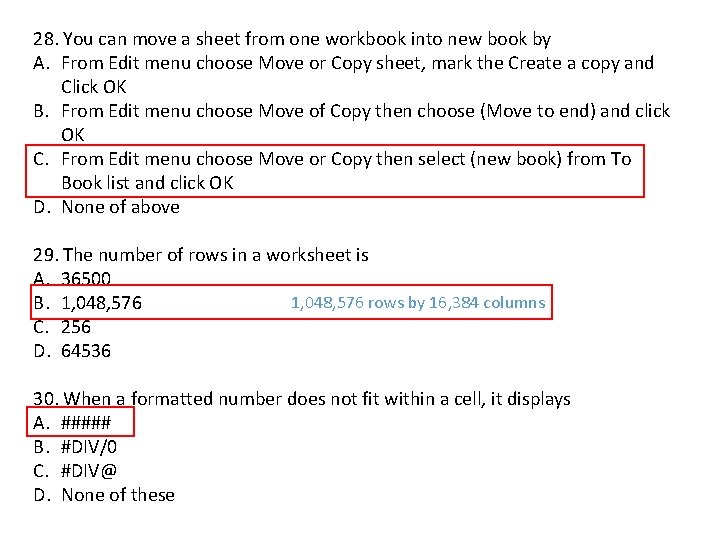
28. You can move a sheet from one workbook into new book by A. From Edit menu choose Move or Copy sheet, mark the Create a copy and Click OK B. From Edit menu choose Move of Copy then choose (Move to end) and click OK C. From Edit menu choose Move or Copy then select (new book) from To Book list and click OK D. None of above 29. The number of rows in a worksheet is A. 36500 1, 048, 576 rows by 16, 384 columns B. 1, 048, 576 C. 256 D. 64536 30. When a formatted number does not fit within a cell, it displays A. ##### B. #DIV/0 C. #DIV@ D. None of these

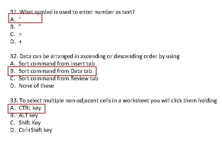
31. What symbol is used to enter number as text? A. ‘ B. " C. = D. + 32. Data can be arranged in ascending or descending order by using A. Sort command from Insert tab B. Sort command from Data tab C. Sort command from Review tab D. None of these 33. To select multiple non-adjacent cells in a worksheet you will click them holding A. CTRL key B. ALT key C. Shift Key D. Ctrl+Shift key

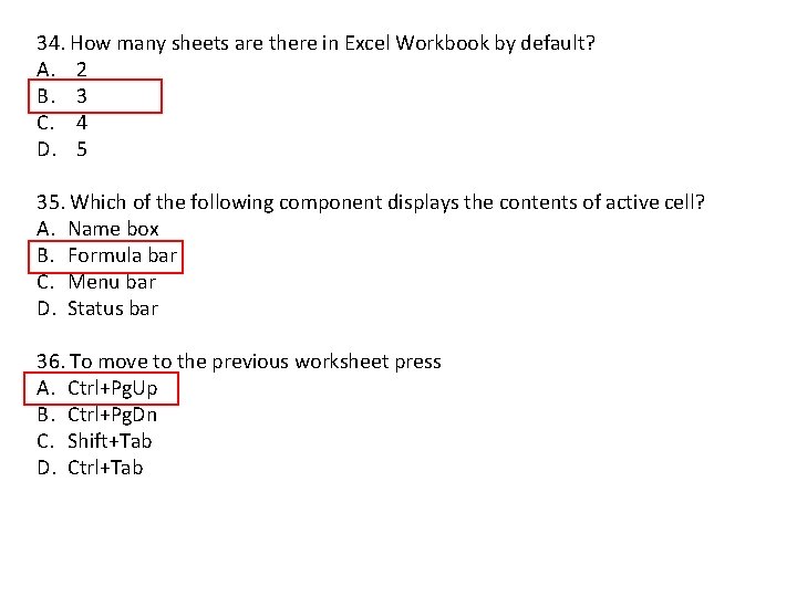
34. How many sheets are there in Excel Workbook by default? A. 2 B. 3 C. 4 D. 5 35. Which of the following component displays the contents of active cell? A. Name box B. Formula bar C. Menu bar D. Status bar 36. To move to the previous worksheet press A. Ctrl+Pg. Up B. Ctrl+Pg. Dn C. Shift+Tab D. Ctrl+Tab

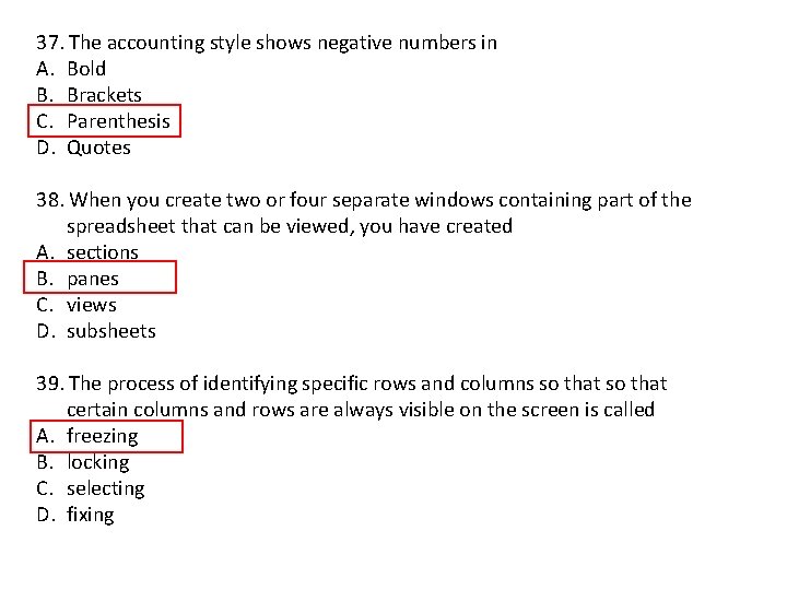
37. The accounting style shows negative numbers in A. Bold B. Brackets C. Parenthesis D. Quotes 38. When you create two or four separate windows containing part of the spreadsheet that can be viewed, you have created A. sections B. panes C. views D. subsheets 39. The process of identifying specific rows and columns so that certain columns and rows are always visible on the screen is called A. freezing B. locking C. selecting D. fixing

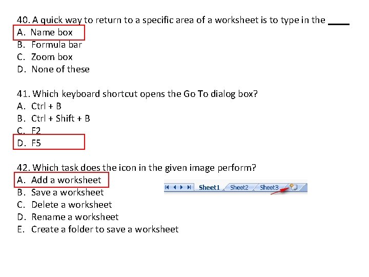
40. A quick way to return to a specific area of a worksheet is to type in the A. Name box B. Formula bar C. Zoom box D. None of these 41. Which keyboard shortcut opens the Go To dialog box? A. Ctrl + B B. Ctrl + Shift + B C. F 2 D. F 5 42. Which task does the icon in the given image perform? A. Add a worksheet B. Save a worksheet C. Delete a worksheet D. Rename a worksheet E. Create a folder to save a worksheet

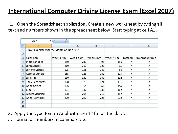
International Computer Driving License Exam (Excel 2007) 1. Open the Spreadsheet application. Create a new worksheet by typing all text and numbers shown in the spreadsheet below. Start typing at cell A 1. 2. Apply the type font in Arial with size 12 for all the data. 3. Format all numbers in comma style.

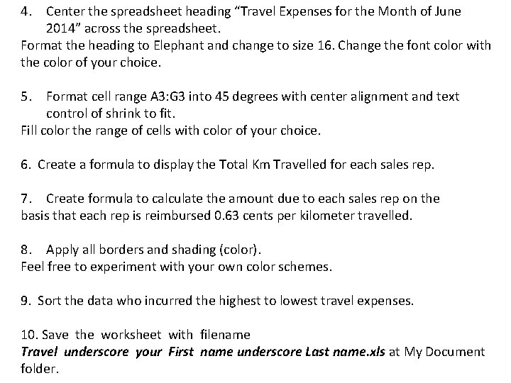
4. Center the spreadsheet heading “Travel Expenses for the Month of June 2014” across the spreadsheet. Format the heading to Elephant and change to size 16. Change the font color with the color of your choice. 5. Format cell range A 3: G 3 into 45 degrees with center alignment and text control of shrink to fit. Fill color the range of cells with color of your choice. 6. Create a formula to display the Total Km Travelled for each sales rep. 7. Create formula to calculate the amount due to each sales rep on the basis that each rep is reimbursed 0. 63 cents per kilometer travelled. 8. Apply all borders and shading (color). Feel free to experiment with your own color schemes. 9. Sort the data who incurred the highest to lowest travel expenses. 10. Save the worksheet with filename Travel underscore your First name underscore Last name. xls at My Document folder.

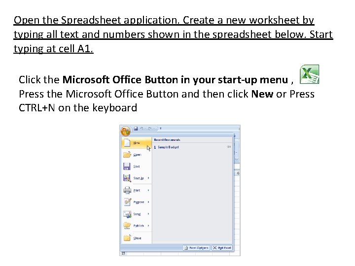
Open the Spreadsheet application. Create a new worksheet by typing all text and numbers shown in the spreadsheet below. Start typing at cell A 1. Click the Microsoft Office Button in your start-up menu , the Press the Microsoft Office Button and then click New or Press CTRL+N on the keyboard

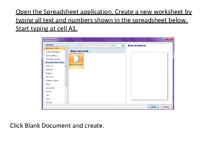
Open the Spreadsheet application. Create a new worksheet by typing all text and numbers shown in the spreadsheet below. Start typing at cell A 1. Click Blank Document and create.

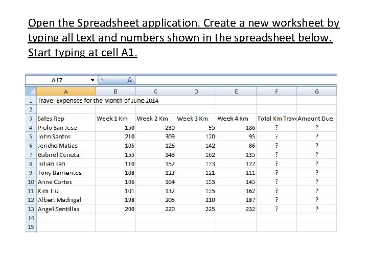
Open the Spreadsheet application. Create a new worksheet by typing all text and numbers shown in the spreadsheet below. Start typing at cell A 1.

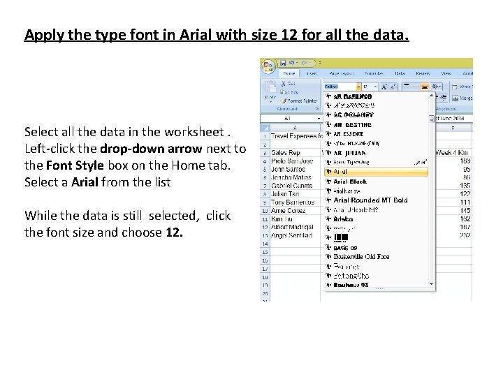
Apply the type font in Arial with size 12 for all the data. Select all the data in the worksheet. Left-click the drop-down arrow next to the Font Style box on the Home tab. Select a Arial from the list While the data is still selected, click the font size and choose 12.

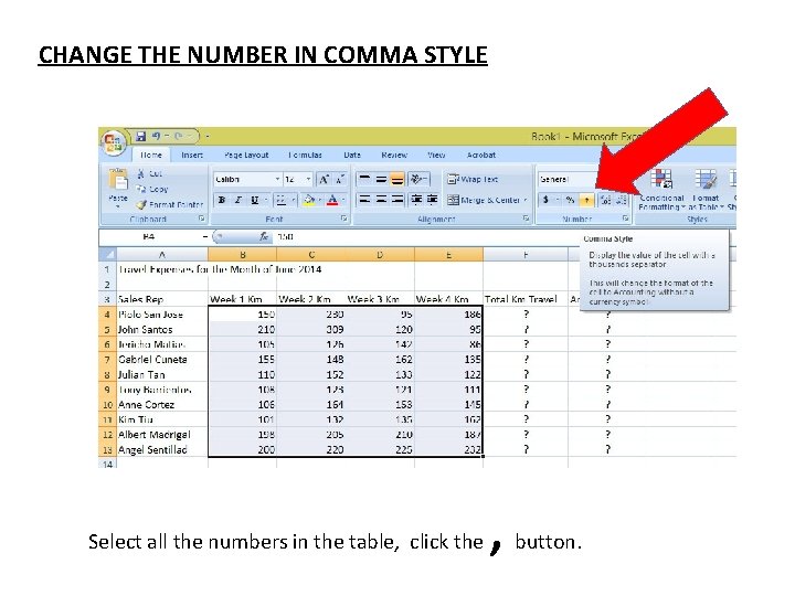
CHANGE THE NUMBER IN COMMA STYLE Select all the numbers in the table, click the , button.

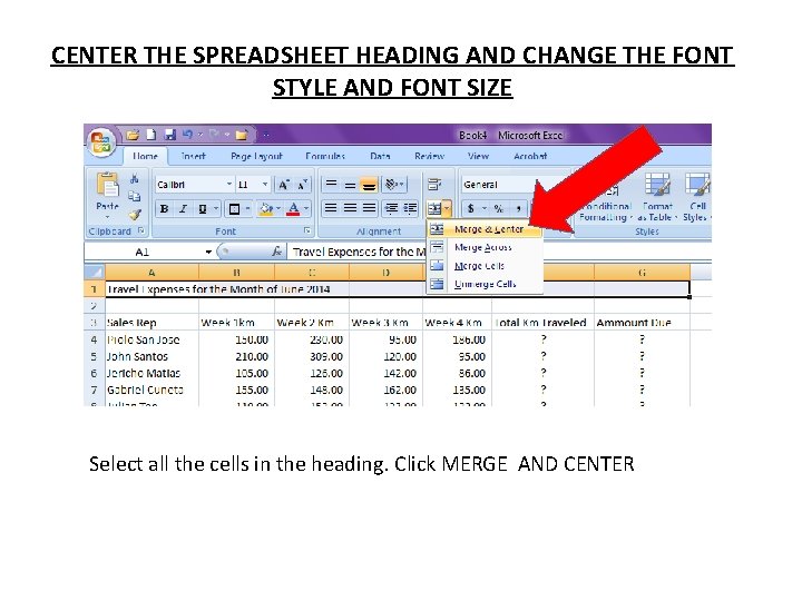
CENTER THE SPREADSHEET HEADING AND CHANGE THE FONT STYLE AND FONT SIZE Select all the cells in the heading. Click MERGE AND CENTER

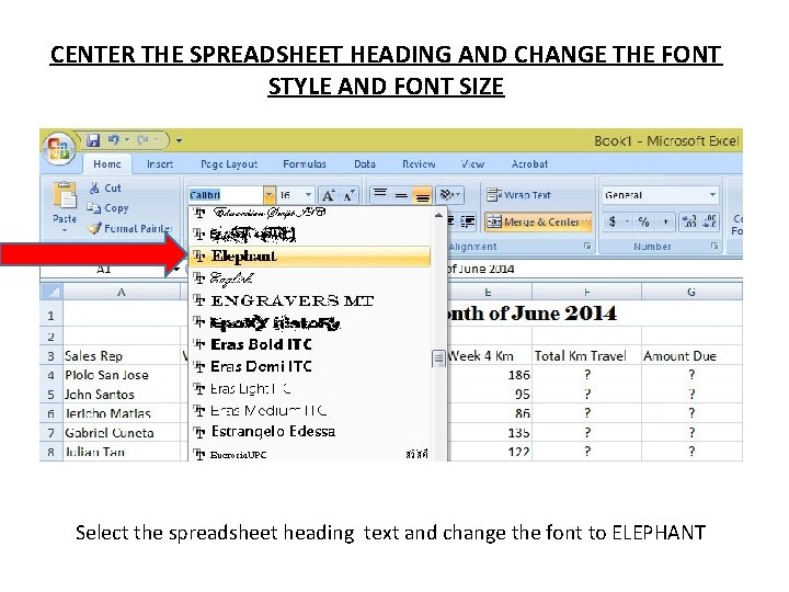
CENTER THE SPREADSHEET HEADING AND CHANGE THE FONT STYLE AND FONT SIZE Select the spreadsheet heading text and change the font to ELEPHANT

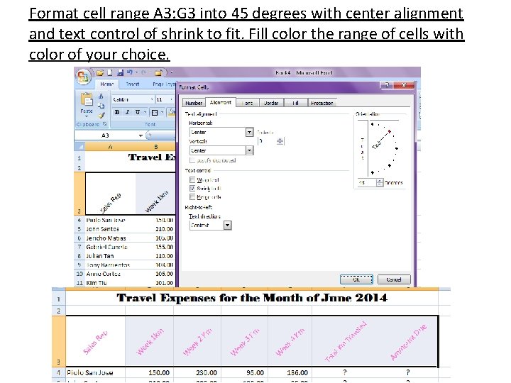
Format cell range A 3: G 3 into 45 degrees with center alignment and text control of shrink to fit. Fill color the range of cells with color of your choice.

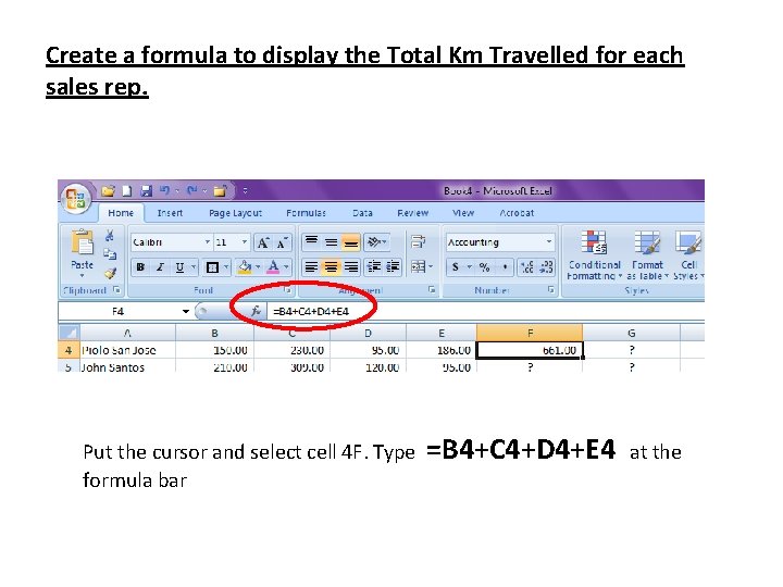
Create a formula to display the Total Km Travelled for each sales rep. Put the cursor and select cell 4 F. Type formula bar =B 4+C 4+D 4+E 4 at the

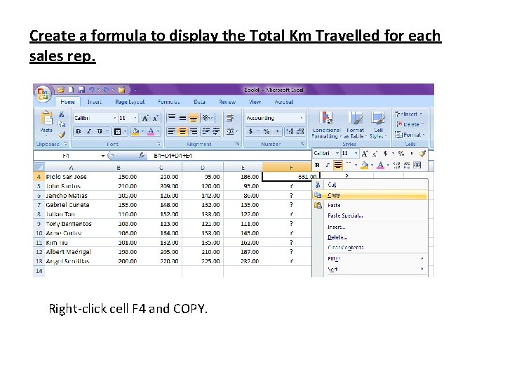
Create a formula to display the Total Km Travelled for each sales rep. Right-click cell F 4 and COPY.

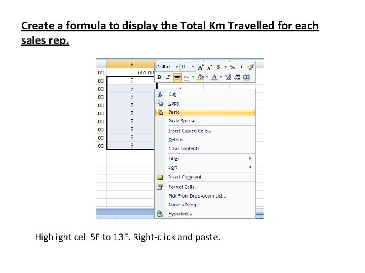
Create a formula to display the Total Km Travelled for each sales rep. Highlight cell 5 F to 13 F. Right-click and paste.

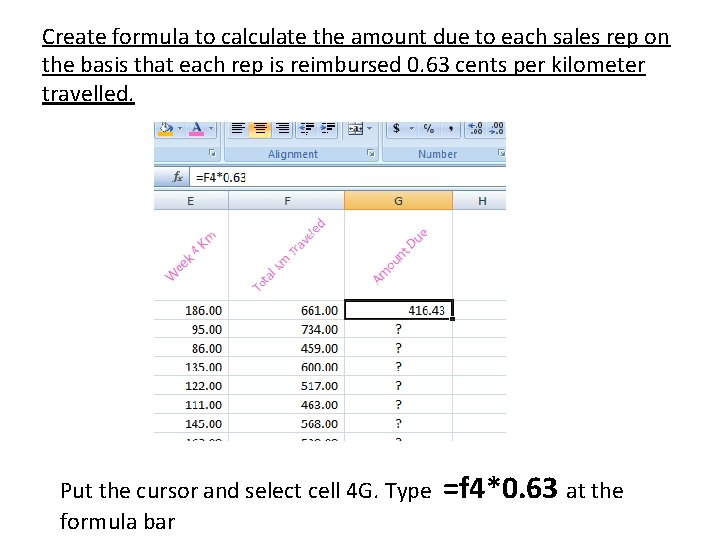
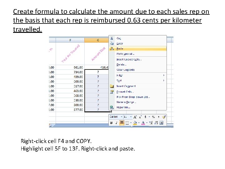
Create formula to calculate the amount due to each sales rep on the basis that each rep is reimbursed 0. 63 cents per kilometer travelled. Put the cursor and select cell 4 G. Type formula bar =f 4*0. 63 at the

Create formula to calculate the amount due to each sales rep on the basis that each rep is reimbursed 0. 63 cents per kilometer travelled. Right-click cell F 4 and COPY. Highlight cell 5 F to 13 F. Right-click and paste.

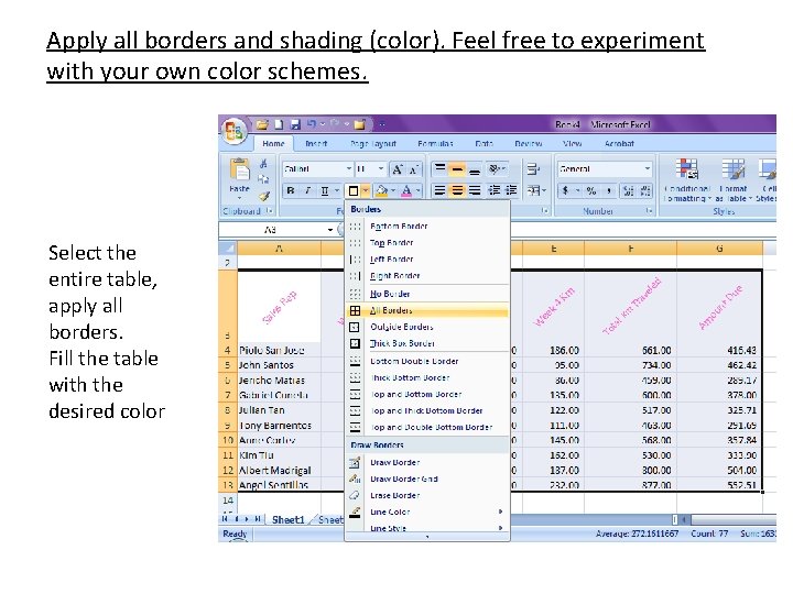
Apply all borders and shading (color). Feel free to experiment with your own color schemes. Select the entire table, apply all borders. Fill the table with the desired color

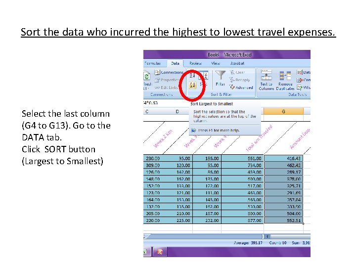
Sort the data who incurred the highest to lowest travel expenses. Select the last column (G 4 to G 13). Go to the DATA tab. Click SORT button (Largest to Smallest)

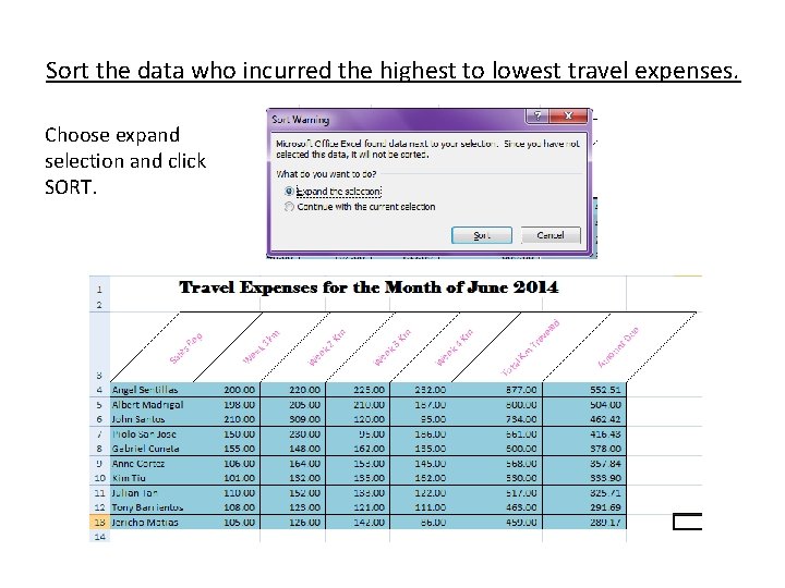
Sort the data who incurred the highest to lowest travel expenses. Choose expand selection and click SORT.

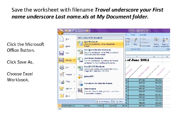
Save the worksheet with filename Travel underscore your First name underscore Last name. xls at My Document folder. Click the Microsoft Office Button. Click Save As. Choose Excel Workbook.

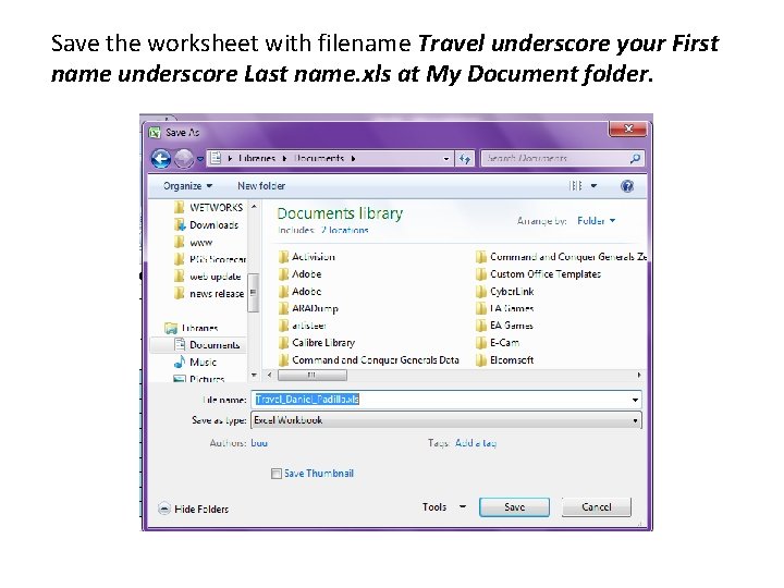
Save the worksheet with filename Travel underscore your First name underscore Last name. xls at My Document folder.