Result of Climate Models Chaithra S T Entry

Result of Climate Models Chaithra S T Entry No: 2019 ASZ 8064

Introduction ● Demonstrating the effect that climate change is having on regional weather is a subject which occupies climate scientists, government policy makers and the media. ● To obtain statistics on the magnitude and frequency of occurrence of extreme weather events, large numbers of simulations of possible weather under the same climate conditions need to be run to assess the odds of such events. ● However, as most extreme weather events occur on a relatively small spatial scale, high-resolution global or regional models are required to realistically capture impact relevant extreme events. ● A recent advancement is the ability to run both a global climate model and a higher resolution regional climate model on a volunteer’s home computer. Such a set-up allows the simulation of weather on a scale that is of most use to studies of the extreme events.

Weather@home ● A new branch of climate science (known as attribution) has sought to quantify how much the risk of extreme events occurring has changed due to climate change. ● One method of attribution uses very large ensembles of climate models computed via volunteer distributed computing. ● The system known as weather@home, by which the global model is coupled to a regional climate model and run on volunteers’ home computers. ● A global climate model that has been developed to simulate the climatology of all major land regions with reasonable accuracy. This then provides the boundary conditions to a regional climate model (which uses the same formulation but at higher resolution) to ensure that it can produce realistic climate and weather over any region of choice.

climateprediction. net ● The largest ensemble climate modelling experiment to date. ● Using distributed volunteer computing, over 126 million years of coupled atmosphere -slab ocean, coupled atmosphere-ocean and medium-resolution atmosphere-only models have been completed. ● weather@home utilises the climateprediction. net volunteer distributed computing network.

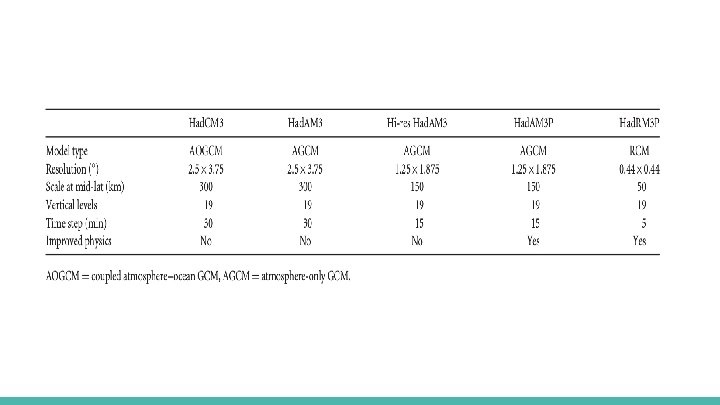
Models used in weather@home ● Had. AM 3 P atmosphere-only global climate model (AGCM) ● Had. RM 3 P regional climate model ● Had. AM 3 P/RM 3 P are based on the Had. CM 3 coupled model. Its atmospheric component, Had. AM 3, forms the basis of this model development ● Had. AM 3 has a latitude-longitude grid of horizontal resolution 2. 5 × 3. 75° with 19 vertical levels (standard resolution) ● 1. 25 × 1. 875° version of Had. AM 3 is called Hi-res Had. AM 3 ● Had. AM 3 P consists of Hi-res Had. AM 3 augmented by a number of changes to the subgrid-scale physics and chemistry.

Calculation of cloud cover ★ In Had. AM 3 the cloud cover and cloud water content in a grid box are both calculated from a saturation variable qc. ★ qc is defined as the difference between total water (i. e. water vapour + liquid + ice) and the saturation vapour pressure (Smith, 1990) ★ Had. AM 3 reproduces the effects of clouds on the global radiation budget quite well, but underestimates cloud cover. ★ Had. AM 3 P address this by introducing a modification in which the cloud scheme is called for three sub-layers within each model grid box, calculating cloud cover from values of qc for each sub-layer obtained by vertical interpolation.

Specification of relative humidity threshold for cloud formation RHcrit - the grid-box mean relative humidity above which cloud begins to form. The assumption that RHcrit does not vary in time or with geographical location is unrealistic. Based on evidence from aircraft observations and high-resolution analyses for numerical weather prediction, Cusack et al. (1999) proposed σ clim (standard deviation of qc within a climate model grid box). σ clim = A(p) ∗ σ 3 × 3 A(p) is a coefficient which varies with pressure model level. σ deviation of qc over neighbouring grid boxes. 3 × 3 is the standard

Improved calculation of the radiative effects of convection ★ Had. AM 3 P includes a set of empirical modifications (Gregory (1999)), which are informed by basic observed properties of anvils as ice clouds which form in the presence of deep convection. When deep convection occurs, the modified scheme increases cloud fraction linearly with height from the freezing level to the cloud top to represent the anvil, and decreases cloud fraction to a constant value below the freezing level to represent the convective tower. If convection is not diagnosed as deep, then no change is made to the calculation of cloud fraction used in Had. AM 3. ★ Simulated convective cloud water amounts are too large in Had. AM 3. The Gregory (1999) modifications address this by reducing the values of cloud water used in the calculation of radiative transfer.

Additional minor changes ★ In Had. AM 3 P vegetated surfaces are assumed to be coupled radiatively to the underlying soil. This weakens the coupling between the ground and surface air temperatures (Best and Hopwood, 2001), leading to an improved diurnal cycle and the removal of unrealistic peaks in the frequency distribution of minimum temperatures associated with soil freezing in winter. ★ Had. AM 3 occasionally simulates unrealistically high surface temperatures in arid regions, because the model only updates radiative fluxes every 3 h, preventing rapid rises in surface temperature driven by strong solar heating from being simultaneously offset by increases in long-wave cooling. ★ In Had. AM 3 P the upward surface long-wave radiation flux is updated every model timestep (15 min), thus removing this unrealistic behaviour.

Experimental design of climate simulations and sensitivity tests ★ Three types of experiments are assessed ★ Sensitivity tests of 18 -42 months to check the effect of changing individual model components. ★ Short, decadal-scale, climatological tests for the period 1980– 1990 to check the effect of multiple changes. ★ Long climate simulations to provide a comprehensive assessment of model performance for the period 1961– 1990. ★ For the sensitivity tests, the first 6 months are used to spin the model up

Set-up of the distributed computing experiment With the increase in computing power, it is now possible to run this model on a home PC, coupled via the lateral boundary conditions to a regional model variant, Had. RM 3 P. Using the distributed computing network of climateprediction. net (CPDN) allows for many thousands of these models to be run on volunteer’s home computers.

Required inputs to the models ★ While running under the distributed network, Had. AM 3 P/RM 3 P requires a number of inputs, which must be supplied to the volunteers’ computers. ★ These include the initial condition of the model and, as the model is atmosphere-only, forcings are required at the sea-surface boundary, in the form SST and sea-ice fraction (SIF). ★ Atmospheric concentrations of the well-mixed greenhouse gases are required, including carbon dioxide (CO 2 ), nitrous oxide (N 2 O), methane (CH 4 ) and the halocarbons. ★ Ozone (O 3) concentrations are required as zonal averages at each model level and the inputs to the sulphur cycle are also required.

Distributed computing ★ To enable the computation of large ensembles of the GCM and RCM, volunteer distributed computing (VDC) is used. ★ Each volunteer signs up to the CPDN project via the BOINC client software, which then downloads the GCM and RCM to the volunteer’s computer. CPDN scientists control the project’s servers, which hand out workunits to volunteers’ client computers. Each workunit contains all the information needed by the climate models to run an experiment for a certain period of model time, under a specified climate scenario. ★ weather@home builds upon CPDN’s success to use the same infrastructure to compute large-ensemble simulations using the Had. AM 3 P/RM 3 P models.

Model coupling ★ Under weather@home, Had. AM 3 P/RM 3 P run on the same client computer in an interleaved manner. ★ The GCM (Had. AM 3 P) runs first for one full model day, providing the lateral boundary conditions (LBCs) to the RCM (Had. RM 3 P) which also runs for one full model day. ★ The coupling between the GCM and RCM is strictly one-way, in that the GCM feeds the RCM but there is no feedback from the RCM to the GCM. ★ The main variables comprising the LBCs are atmospheric pressure at the surface along with horizontal winds, temperature and humidity for all atmospheric layers.

Model initial conditions ★ The distributed system runs the Had. AM 3 P/RM 3 P models for 1 year at a time, in a time-slice manner. ★ In order to produce a timeseries of integrated models, a continuation system is used. Initially, the project creates a pool of workunits, each with the same generic starting conditions, at 5 -yearly intervals. ★ These workunits are handed out to client computers, integrated over the model year under the specified climate scenario, and the results from the integration are returned, along with the final state of the model. ★ This final state is then incorporated into a new workunit describing the next year of the climate scenario, using this final state as the starting condition. ★ This process is repeated with the final states of the subsequent integrations, enabling a time series of climate model integrations to be built from the single-year runs.

Forcings at the (sea) surface ★ SSTs and SIFs are defined per grid box for the GCM, with the RCM using the same field interpolated to the finer grid. ★ Had. ISST 1 (Rayner et al. , 2003) is used to provide both the SST and SIF fields. Had. ISST has been specifically designed to drive atmospheric climate models. ★ Had. ISST is provided as a global coverage dataset (non-land points only) as monthly means(1°× 1°). In order to use these data to drive the Had. AM 3 P/RM 3 P model, they must be regridded to the GCM resolution of 1. 875 × 1. 25° (area-weighted averaging method). ★ Assigning any grid box where missing data occurs with the mean of the surrounding grid boxes which themselves do not have missing data. ★ In addition to the spatial regridding, the Had. ISST data are also temporally regridded.

Atmospheric composition ★ The concentrations of CO 2, CH 4 and N 2 O follow the timeseries of the observed quantities in the IPCC Fourth Assessment Report. ★ The halocarbon gases (CFC 113, CFC 11, CFC 12, HCFC 22, HFC 124 and HFC 134 A) are represented as a single value per time point in the timeseries, which produces the equivalent radiative forcing as if all six gases were modelled. ★ Ozone (O 3) also follows the observations from AR 4, including the appearance of the ozone hole in the 1980 s.

Additional climate drivers ★ An extra modification to Had. AM 3 P/RM 3 P for weather@home is the addition of large -scale volcanic eruptions emitting large quantities of SO 2. ★ These large natural emissions are modelled in four latitude bands, with a value prescribed for each band for each model year. ★ weather@home also applies a small modification to Had. AM 3 P to account for variations in solar activity by allowing anomalies from the solar constant to be specified. ★ These anomalies take into account the 11 year solar cycle as well as longer time-scale solar processes. (Krivova et al. (2007))

Results from the distributed computing experiment ★ Using the experimental set-up, approximately 500 ensemble members per year have been computed, for the historical period of 1961– 1990. ★ The large ensemble capacity of weather@home is of most use when examining extreme weather events which, by their very nature, are rare and require a large ensemble to generate examples of the event. ★ Conversely, to characterise the climatology and overall distribution of climate variables over a 30 year period, a much smaller ensemble is required.