Regional Ocean Modeling System ROMS For the NonSpecialist

Regional Ocean Modeling System (ROMS) For the Non-Specialist (ROMS – LITE) Courtney Harris Virginia Institute of Marine Science Thanks to Julia Moriarty and Tara Kniskern Posted by Irina Overeem, May 2016

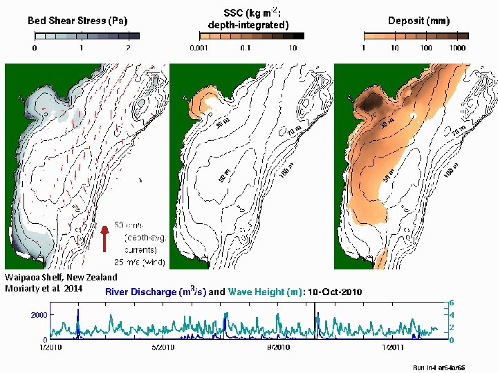
Waipaoa Shelf, New Zealand Moriarty et al. 2014

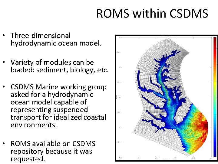
ROMS within CSDMS • Three-dimensional hydrodynamic ocean model. • Variety of modules can be loaded: sediment, biology, etc. • CSDMS Marine working group asked for a hydrodynamic ocean model capable of representing suspended transport for idealized coastal environments. • ROMS available on CSDMS repository because it was requested.

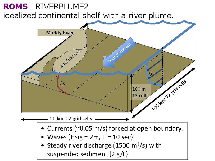
Outline • Overview the ROMS model framework and input / output. • Demonstrate an idealized continental shelf model. • Learn to browse model results. • Learn to modify the test case and re-run it.

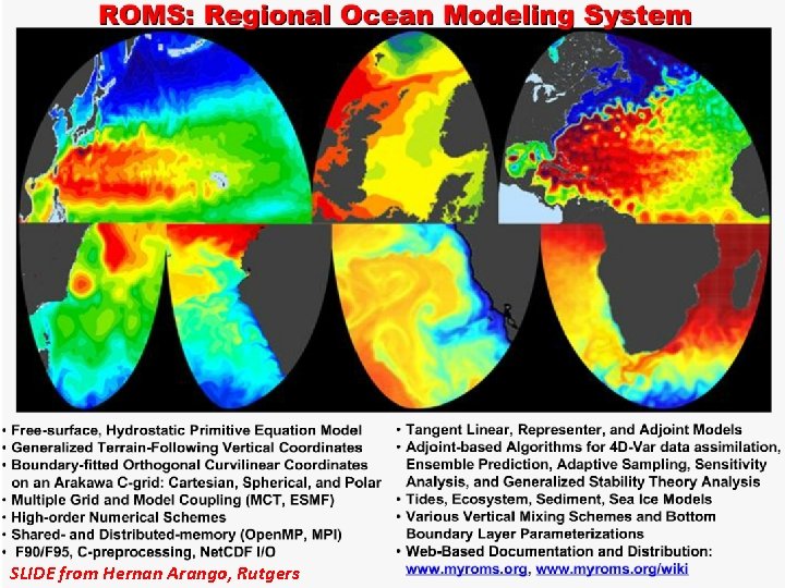
SLIDE from Hernan Arango, Rutgers

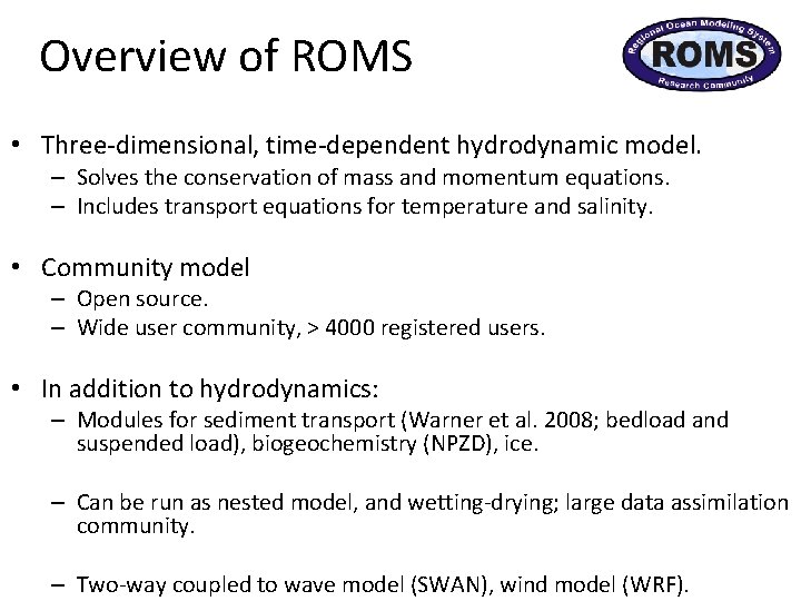
Overview of ROMS • Three-dimensional, time-dependent hydrodynamic model. – Solves the conservation of mass and momentum equations. – Includes transport equations for temperature and salinity. • Community model – Open source. – Wide user community, > 4000 registered users. • In addition to hydrodynamics: – Modules for sediment transport (Warner et al. 2008; bedload and suspended load), biogeochemistry (NPZD), ice. – Can be run as nested model, and wetting-drying; large data assimilation community. – Two-way coupled to wave model (SWAN), wind model (WRF).

Overview of ROMS, cont. • Features of the code: – Written in Fortran-90 – Parallelized (MPI). – Includes sets of options: advection schemes, turbulence closures, bottom boundary layer treatments. – Output: Net. CDF “history” file, ocean_his_*. nc. – Input: format is a somewhat flexible (confusing? ) mix of Net. CDF, text files, and some hard-wiring.

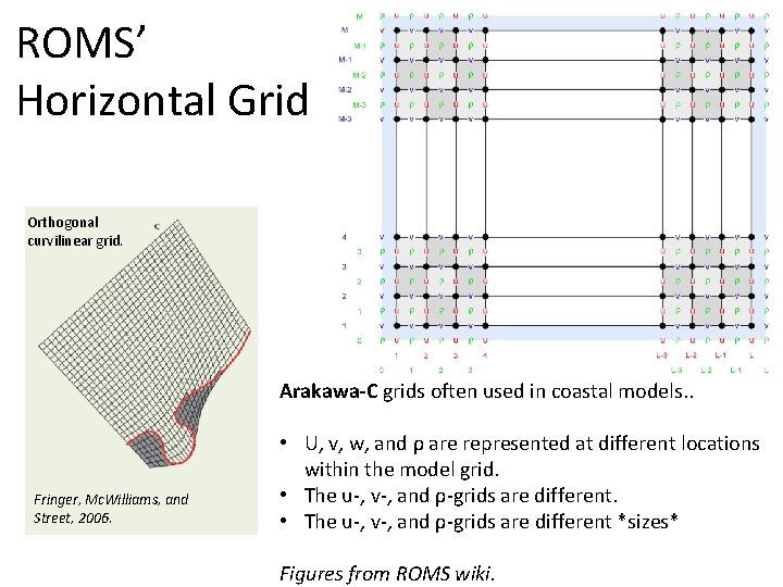
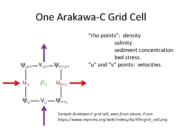
ROMS’ Horizontal Grid Orthogonal curvilinear grid. Arakawa-C grids often used in coastal models. . Fringer, Mc. Williams, and Street, 2006. • U, v, w, and ρ are represented at different locations within the model grid. • The u-, v-, and ρ-grids are different *sizes* Figures from ROMS wiki.

One Arakawa-C Grid Cell “rho points”: density salinity sediment concentration bed stress. “u” and “v” points: velocities. Sample Arakawa-C grid cell, seen from above. From https: //www. myroms. org/wiki/index. php/File: grid_cell. png

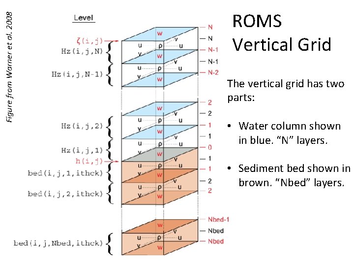
Figure from Warner et al. 2008 ROMS Vertical Grid The vertical grid has two parts: • Water column shown in blue. “N” layers. • Sediment bed shown in brown. “Nbed” layers.

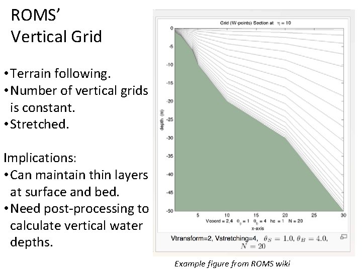
ROMS’ Vertical Grid • Terrain following. • Number of vertical grids is constant. • Stretched. Implications: • Can maintain thin layers at surface and bed. • Need post-processing to calculate vertical water depths. Example figure from ROMS wiki

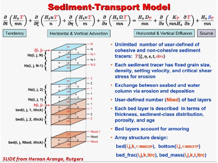
SLIDE from Hernan Arango, Rutgers

ROMS RIVERPLUME 2 idealized continental shelf with a river plume. Muddy River it s o ep d lf e sh Cs u rre m 5 c c /s nt v s 100 m 13 cells rid g 2 ll ce ; 7 0 10 km 50 km; 52 grid cells • Currents (~0. 05 m/s) forced at open boundary. • Waves (Hsig = 2 m, T = 10 sec) • Steady river discharge (1500 m 3/s) with suspended sediment (2 g/L).

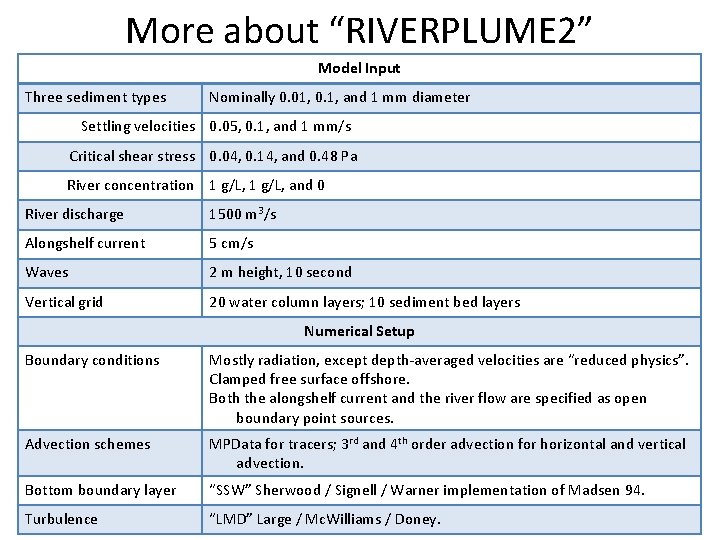
More about “RIVERPLUME 2” Model Input Three sediment types Nominally 0. 01, 0. 1, and 1 mm diameter Settling velocities 0. 05, 0. 1, and 1 mm/s Critical shear stress 0. 04, 0. 14, and 0. 48 Pa River concentration 1 g/L, and 0 River discharge 1500 m 3/s Alongshelf current 5 cm/s Waves 2 m height, 10 second Vertical grid 20 water column layers; 10 sediment bed layers Numerical Setup Boundary conditions Mostly radiation, except depth-averaged velocities are “reduced physics”. Clamped free surface offshore. Both the alongshelf current and the river flow are specified as open boundary point sources. Advection schemes MPData for tracers; 3 rd and 4 th order advection for horizontal and vertical advection. Bottom boundary layer “SSW” Sherwood / Signell / Warner implementation of Madsen 94. Turbulence “LMD” Large / Mc. Williams / Doney.

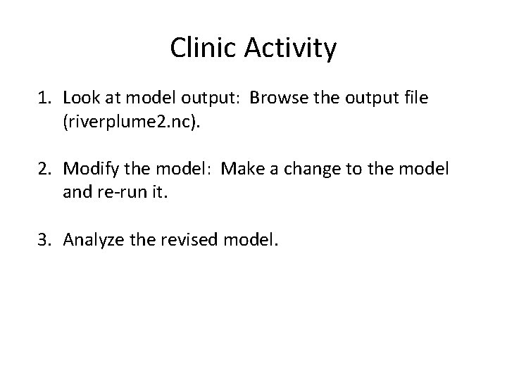
Clinic Activity 1. Look at model output: Browse the output file (riverplume 2. nc). 2. Modify the model: Make a change to the model and re-run it. 3. Analyze the revised model.

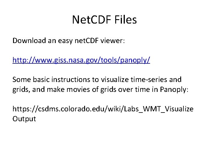
Net. CDF Files Download an easy net. CDF viewer: http: //www. giss. nasa. gov/tools/panoply/ Some basic instructions to visualize time-series and grids, and make movies of grids over time in Panoply: https: //csdms. colorado. edu/wiki/Labs_WMT_Visualize Output

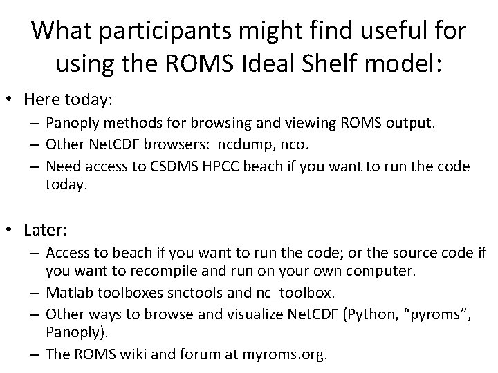
What participants might find useful for using the ROMS Ideal Shelf model: • Here today: – Panoply methods for browsing and viewing ROMS output. – Other Net. CDF browsers: ncdump, nco. – Need access to CSDMS HPCC beach if you want to run the code today. • Later: – Access to beach if you want to run the code; or the source code if you want to recompile and run on your own computer. – Matlab toolboxes snctools and nc_toolbox. – Other ways to browse and visualize Net. CDF (Python, “pyroms”, Panoply). – The ROMS wiki and forum at myroms. org.

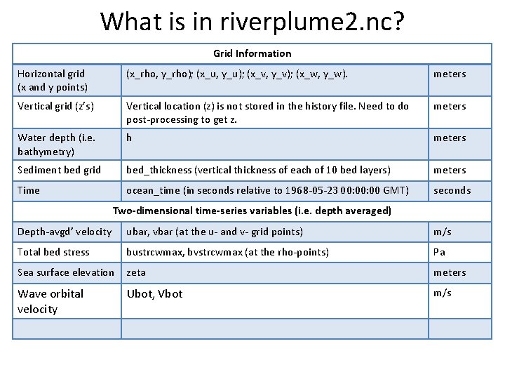
What is in riverplume 2. nc? Grid Information Horizontal grid (x and y points) (x_rho, y_rho); (x_u, y_u); (x_v, y_v); (x_w, y_w). meters Vertical grid (z’s) Vertical location (z) is not stored in the history file. Need to do post-processing to get z. meters Water depth (i. e. bathymetry) h meters Sediment bed grid bed_thickness (vertical thickness of each of 10 bed layers) meters Time ocean_time (in seconds relative to 1968 -05 -23 00: 00 GMT) seconds Two-dimensional time-series variables (i. e. depth averaged) Depth-avgd’ velocity ubar, vbar (at the u- and v- grid points) m/s Total bed stress bustrcwmax, bvstrcwmax (at the rho-points) Pa Sea surface elevation zeta meters Wave orbital velocity Ubot, Vbot m/s

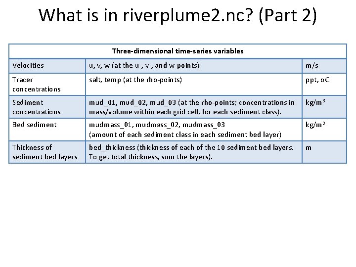
What is in riverplume 2. nc? (Part 2) Three-dimensional time-series variables Velocities u, v, w (at the u-, v-, and w-points) m/s Tracer concentrations salt, temp (at the rho-points) ppt, o. C Sediment concentrations mud_01, mud_02, mud_03 (at the rho-points; concentrations in mass/volume within each grid cell, for each sediment class). kg/m 3 Bed sediment mudmass_01, mudmass_02, mudmass_03 (amount of each sediment class in each sediment bed layer) kg/m 2 Thickness of sediment bed layers bed_thickness (thickness of each of the 10 sediment bed layers. To get total thickness, sum the layers). m

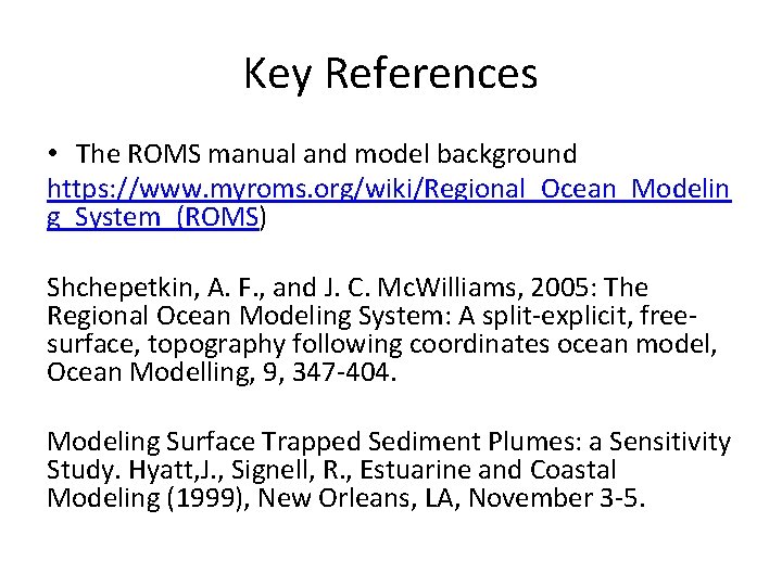
Key References • The ROMS manual and model background https: //www. myroms. org/wiki/Regional_Ocean_Modelin g_System_(ROMS) Shchepetkin, A. F. , and J. C. Mc. Williams, 2005: The Regional Ocean Modeling System: A split-explicit, freesurface, topography following coordinates ocean model, Ocean Modelling, 9, 347 -404. Modeling Surface Trapped Sediment Plumes: a Sensitivity Study. Hyatt, J. , Signell, R. , Estuarine and Coastal Modeling (1999), New Orleans, LA, November 3 -5.