Redshift Estimation and Photometric Classification of SDSS Quasars

SDSS J 1106+1939 Twinkle, twinkle, quasi-star, Biggest puzzle from afar. How unlike the other

• Quasars are the most active galactic nucleus (very high luminosity) • Nowadays,

Roadmap • Dataset: SDSS Quasar Catalog Tenth Release • Random Forest to estimate redshifts

http: //iopscience. iop. org/article/10. 1088 /0004 -637 X/712/1/511/pdf

Photo-z Regression u g r i z Spec-z ↓ ↓ ↓ Quasar 1 Quasar

1) IF we look at the first four bins (equal size N = 40,

2) We can use high emission lines to guide expectation for most important band

2) For a given bin, have range of redshift and corresponding wavelength range we

Outliers Exp. m. i. b. = g Calc. m. i. b. = u

Classification • Unsupervised classification: Ø Self-Organizing Map classifies objects by photometry into minimum number

Plot of r vs u bands All other bands produce similar structure

Slides: 19

Download presentation

Redshift Estimation and Photometric Classification of SDSS Quasars Nathan Steinle UTD Physics Department

SDSS J 1106+1939 Twinkle, twinkle, quasi-star, Biggest puzzle from afar. How unlike the other ones, Brighter than a trillion Suns. Twinkle, twinkle, quasi-star, How I wonder what you are! - George Gamow Exploring the Cosmos, Louis Berman, Ch. 14, pg. 311, 1973 https: //scitechdaily. com/scientists-discover-the-most-powerful-quasar-outflow-ever/

• Quasars are the most active galactic nucleus (very high luminosity) • Nowadays, very large data sets: Ø Advanced Statistics Ø Big Data Ø Machine Learning Centaurus A http: //math. ucr. edu/home/baez/doomed. html

Roadmap • Dataset: SDSS Quasar Catalog Tenth Release • Random Forest to estimate redshifts using photometric data Ø which inputs are most important? • Use Self-Organizing Map for photometric classification Ø how are the quasars related by their photometry?

http: //iopscience. iop. org/article/10. 1088 /0004 -637 X/712/1/511/pdf

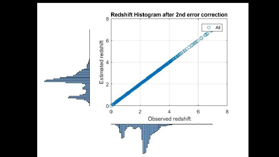
Photo-z Regression u g r i z Spec-z ↓ ↓ ↓ Quasar 1 Quasar 2 Quasar 3 I. Split quasars into 6 bins according to redshift: 0 – 1. 95 1. 95 – 2. 34 2. 34 – 2. 63 2. 63 – 3. 5 3. 5 – 4. 5 4. 5 – 7. 11 Ø In each bin, have training set and indep. testing set. II. Iterative error-reduction truth vs estimate scatter diagrams Spec-z Photo-z III. Ranking of inputs by relative importance

Bin 1

Bin 2

1) IF we look at the first four bins (equal size N = 40, 000), we expect them to have different “most important band” (m. i. b. )

2) We can use high emission lines to guide expectation for most important band (m. i. b. ) In rest frame (lab) Lyα emission line is at 1215. 67 Å Cosmological redshift: This means I expect to observe the Lyα line in the r band http: //classic. sdss. org/gallery/gal_spectra. html Z = 4. 16 quasar

2) For a given bin, have range of redshift and corresponding wavelength range we expect to find Lyα Bin # Z-spec range Expected Lyα range (Å) Expected m. i. b. Calculated m. i. b. 1 0 – 1. 95 1215 – 3587 u u 2 1. 95 – 2. 34 3587 – 4061 u/g u 3 2. 34 – 2. 63 4061 – 4416 g u 4 2. 63 – 3. 5 4416 – 5470 g u 5 3. 5 – 4. 5 5470 – 6686 g/r g 6 4. 5 – 7. 01 6686 - 9738 i i

Outliers Exp. m. i. b. = g Calc. m. i. b. = u

Classification • Unsupervised classification: Ø Self-Organizing Map classifies objects by photometry into minimum number of classes

Plot of r vs u bands All other bands produce similar structure

Thank you for listening!