Prof George Halkos and Asst Prof Nickolaos Tzeremes

Prof. George Halkos and Asst Prof. Nickolaos Tzeremes Laboratory of Operations Research, Department of Economics, University of Thessaly, Korai 43, 38333 Volos, Greece E-mail : halkos@econ. uth. gr The effect of electricity consumption from renewable sources on countries’ economic growth levels: Evidence from advanced, emerging and developing economies. 1

Energy consumption and economic growth hypotheses • Growth hypothesis implies a unidirectional hypothesis causality from energy consumption to economic growth. • Conservation hypothesis describes a unidirectional causality from economic growth to energy consumption. • Feedback hypothesis supports the bidirectional hypothesis causality among energy consumption and economic growth. • Neutrality hypothesis describes the case where energy consumption has no significant effect on economic growth. 2

Energy consumption and economic growth • The results of the causal relationship are rather mixed failing to establish most of the time the same relationship (Soytas and Sari 2006, 2007). • This is mainly due to: Different methodologies applied, Different samples, Different examined periods, and Different countries’ development stages (Yuan et al. , 2008; Halkos and Tzeremes, 2009). 3

Electricity consumption/generation and economic growth • Ghosh (2002) found a unidirectional causality relationship from economic growth to electricity consumption in the case of India (for the short-run). • Ghosh (2009) for the time span of 1970 -1971 to 20052006 in the case of India investigated the relationship between electricity supply, employment and real GDP. • Altinay and Karagol (2005) found causality relationship running from income to electricity consumption in the case of Turkey. • Similarly, Aqeel and Butt (2001) found same relationship for Pakistan, Jumbe (2004) for Malawi, Shiu and Lam (2004) for China and Murry and Nan (1996) for East Asian countries. 4

This study • • • It is based on the growth hypothesis analyzing the effect of electricity hypothesis consumption from renewable sources (REN) on countries' economic growth levels. We use a sample of total 36 countries- Time period 1990 -2011 (792 observations per variable) Advanced-developed countries (23): Australia, Belgium, Canada, Czech Republic, Denmark, Finland, France, Germany, Greece, Italy, Ireland, Japan, Korea Republic of, Netherlands, New Zealand, Norway, Portugal, Spain, Sweden, Switzerland, Taiwan, United Kingdom and the United States of America. Emerging market-developing countries (13): Argentina, Brazil, Chile, China, Colombia, Hungary, India, Indonesia, Mexico, Philippines, Poland, Russia, Turkey (IMF Advanced Economies List, 2012, p. 179 -183). Dependent variable: Real GDP PPP (in m 2005 US $) as dependent variable Penn World Table-PWT 8. 0 (Feenstra et al. , 2013). Independent variable: Electricity consumption (in TWh) derived from renewable sources including wind, geothermal, solar, biomass and waste, and not accounting for cross border electricity supply (Statistical Review of World Energy). 5

Nonparametric regression analysis • Regression is probably the most popular technique based on data to examine the interaction between variables, especially in cases described as ‘‘cause and effect’’. In general, a linear model is postulated, without accounting too much for the mechanism underlying the relationship being modelled. • the assumption of statistical adequacy, or correct specification of the model has traditionally been a major concern, and an incorrect specification of the functional forms can imply invalid tests for the hypothesis under analysis. 6

Nonparametric regression analysis • Nonparametric regression allows us to graphically observe how a certain Y variable (GDP) and each of its components, is affected by changes in another variable X (electricity consumption from renewable sources, RE). • To avoid mixing notation, dependent variable Y will be labelled GDP whereas independent variable(s) will be referred to as Z(RE). • The main advantage of this technique, as opposed to others such as linear or Local Linear (LL) regression, lies in the fact that it does not impose any type of a priori relationship between the variables analyzed. 7

Nonparametric regression analysis • Therefore, cases in which nonparametric regression is more useful are those in which it is not possible to know the nature of m, i. e. , it is impossible to know whether the relation is linear, quadratic, growing in Z, etc. • The basic idea is to obtain the mean of GDP conditioned on a certain value of RE, for example REi, defining an interval around this value and computing a weighted mean of values GDP that correspond to the observations within the interval. • It is therefore, a local averaging procedure where the local average is constructed in such a way that is defined only from observations in a small area 8 around RE.

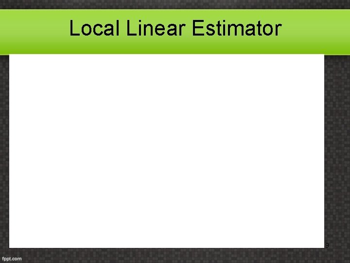
Local Linear Estimator 9

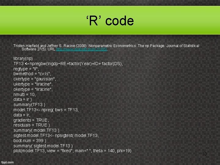
‘R’ code Tristen Hayfield and Jeffrey S. Racine (2008). Nonparametric Econometrics: The np Package. Journal of Statistical Software 27(5). URL http: //www. jstatsoft. org/v 27/i 05/. library(np) TF 13 <- npregbw(lngdp~RE+factor(Year)+ID+ factor(DS), regtype = "ll", bwmethod = "cv. ls", ckertype = "gaussian", ukertype = "liracine", okertype = "liracine", nmulti = 10, data = lr ) summary(TF 13 ) model. TF 13<- npreg( bws = TF 13, data = lr, gradients = TRUE, residuals = TRUE ) summary( model. TF 13 ) sigtest. model. TF 13<- npsigtest( model. TF 13, boot. num = 399 ) summary( sigtest. model. TF 13 ) plot(model. TF 13, view = "fixed", main=" ", theta = 140, phi=19) 10

Diachronical representation of the variables 11

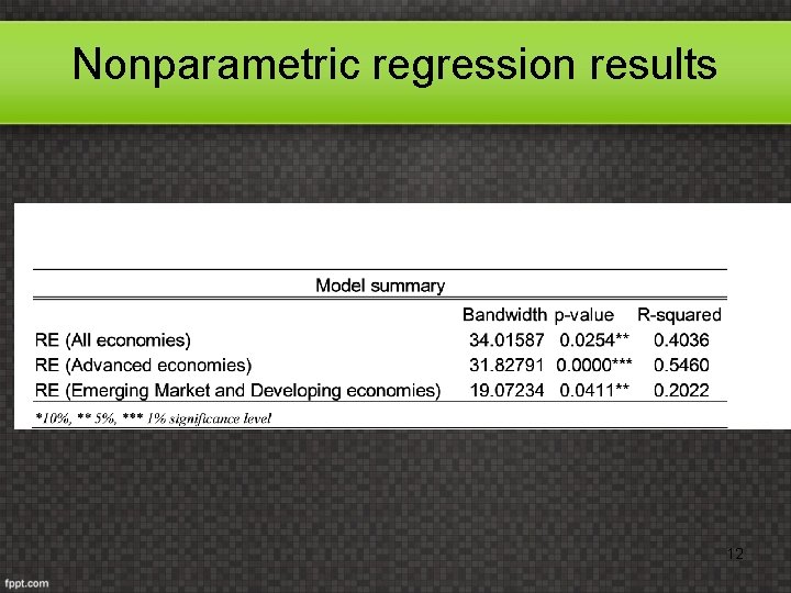
Nonparametric regression results 12

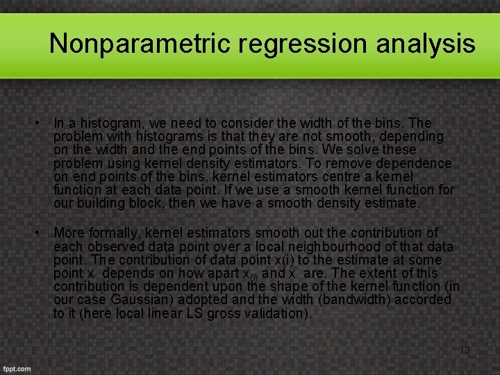
Nonparametric regression analysis • In a histogram, we need to consider the width of the bins. The problem with histograms is that they are not smooth, depending on the width and the end points of the bins. We solve these problem using kernel density estimators. To remove dependence on end points of the bins, kernel estimators centre a kernel function at each data point. If we use a smooth kernel function for our building block, then we have a smooth density estimate. • More formally, kernel estimators smooth out the contribution of each observed data point over a local neighbourhood of that data point. The contribution of data point x(i) to the estimate at some point x depends on how apart x(i) and x are. The extent of this contribution is dependent upon the shape of the kernel function (in our case Gaussian) adopted and the width (bandwidth) accorded to it (here local linear LS gross validation). 13

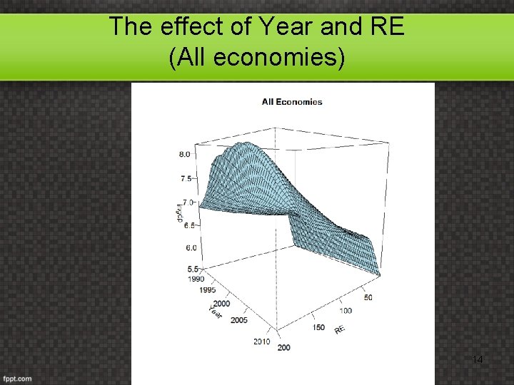
The effect of Year and RE (All economies) 14

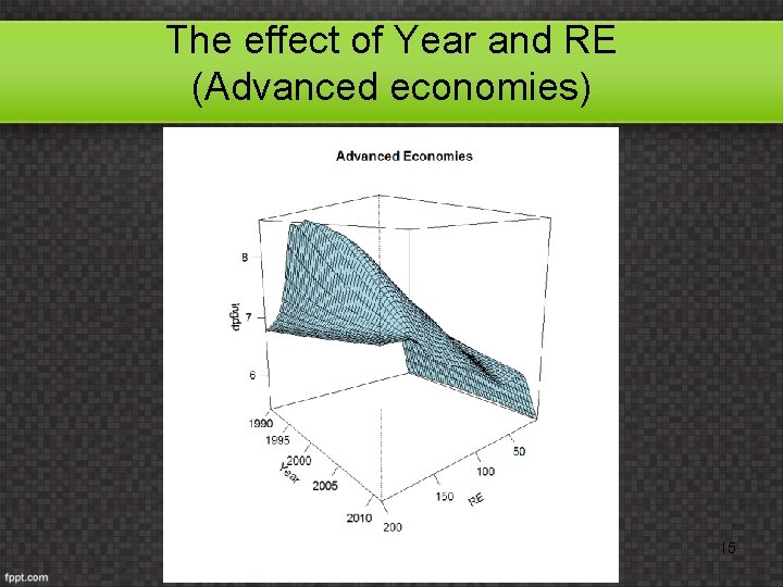
The effect of Year and RE (Advanced economies) 15

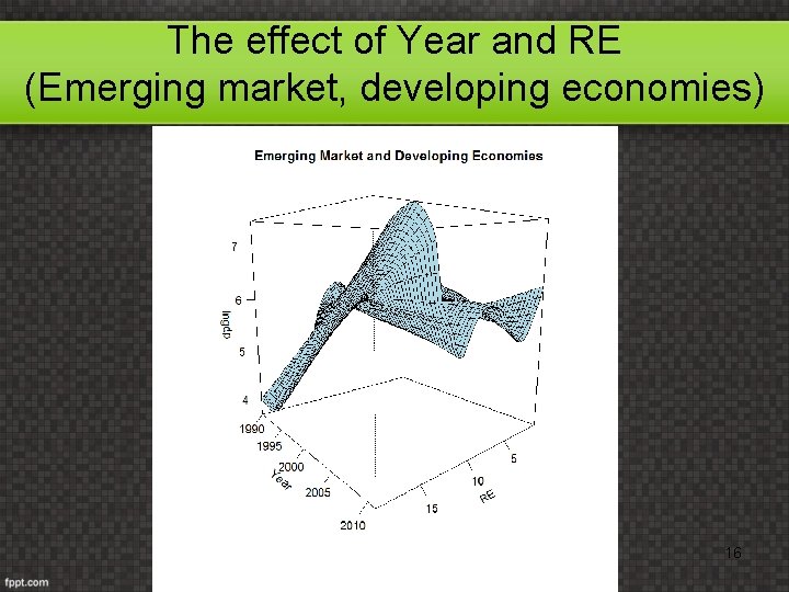
The effect of Year and RE (Emerging market, developing economies) 16

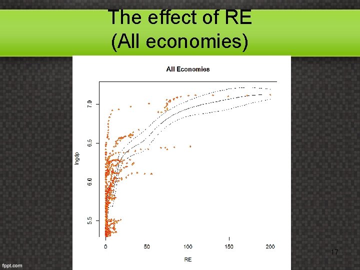
The effect of RE (All economies) 17

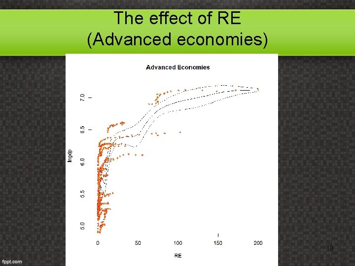
The effect of RE (Advanced economies) 18

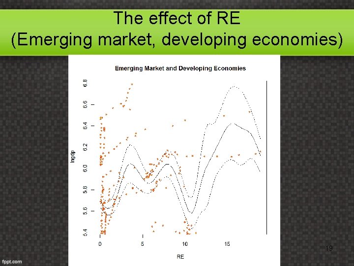
The effect of RE (Emerging market, developing economies) 19

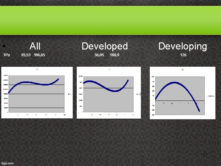
Findings • The growth hypothesis is verified. hypothesis • All the economies: The results reveal that time (Year) has a positive effect on countries' GDP levels alongside with RE. • Advanced economies: The results reveal that time (Year) has a positive effect on countries' GDP levels alongside with RE. • Emerging markets, developing economies: The effect of time is highly positive for developing countries' GDP levels. An 'M' shape up to a consumption level of 10 terawatts per hour. For greater electricity consumption levels an inverted 'U' shape is reported. 20

Why is that for the developing countries? • Barriers and lack of implementation of renewable sources (among others Beck and Marinot, 2004): a) Costs and pricing issues: RE costs more than other energy sources cost-driven decisions and policies to avoid RE. Life cycle costs account initial capital costs, future fuel and O and M costs, equipment lifetime b) Legal and regulatory policies: In many cases power utilities still control a monopoly on electricity production and distribution. In such cases independent power producers may be unable to invest in RE c) Market performance factors 21

Barriers related to cost and pricing • Subsidies for competing fuels: Public subsidies may take the form of direct budgetary transfers, tax incentives, R&D, liability insurance, waste disposal etc. Large subsidies on FFs may lower substantially final energy prices competitive disadvantage for RE • High initial capital costs: Lower fuel and O and M costs may give a cost advantage to RE high initial capital costs may imply a burden (less installed capacity per $ invested compared to conventional energy sources) • Difficulty of fuel price risk assessment: Risks related to variability of future FFs’ prices difficult to assess and possible ignored in initial decision making • Unfavourable power pricing rules • Transaction costs: May make RE more expensive. In RE we may have resource assessment, sitting, permitting, developing project proposals, assembling financial packages etc may be much higher on a k. W capacity basis for conventional power plants. • Environmental externalities: Effects of FFs social costs 22

Barriers related to legal and regulatory aspects • Restriction on sitting and construction: Wind turbines may create problems in birds paths or coastal zones; photovoltaic installations, biomass combustion etc may face building restrictions due to height, noise, aesthetics mainly in urban areas. • Transmission access: This is an important determinant as some RE sources may be located far from populated areas. • Utility interconnection requirements: Lack of uniform requirements may increase transaction costs and transaction costs of hiring legal and technical staff to understand comply with interconnection requirements may be substantial, The need for appropriate policies to create sound and uniform interconnection standards crucial. • Liability insurance requirements: Small power generators (like home photovoltaic) may have to cope with excessive requirements for liability 23 insurance.

Barriers related to market performance • Lack of access to credit: Consumers or project managers may have limited access to credit to purchase or invest on RE. • Uncertainty and risk related to perceived technology performance: Cost-effective methods may be proceeded as risky if there is little experience with them in a new application or region. • Lack of technical or commercial skills and information: Markets function best when all have low-cost access to good informtion and the necessary skills, . But in many cases skilled personnel who can install, operate and maintain RE may be limited. 24

THANK YOU 25

Panel data methods • First method employed imposes same intercept and slope parameter for all countries (equivalent to OLS estimation). • Second method is the FE allowing each individual country to have a different intercept treating the αi and γt as regression parameters. This practically denotes that the means of each variable for each country are subtracted from the data for that country and the mean for all countries in the sample in each individual time period is also deducted from the observations from that period. Then OLS is used to estimate the regression with the transformed data. • Third model is the RE in which individual effects are treated as random, with αi and γt treated as components of the random disturbances. Residuals from an OLS estimate of the model with a single intercept are used to construct variances utilized in a GLS estimates. • To control for non-observable specific effects 2 SLS was applied but the results were insignificant. 26

• All Developed Developing TPs 93, 53 196, 65 36, 05 188, 9 126 27