Practical Solutions Comparing Proportions Analysing Categorical Data Practical

Practical Solutions Comparing Proportions & Analysing Categorical Data

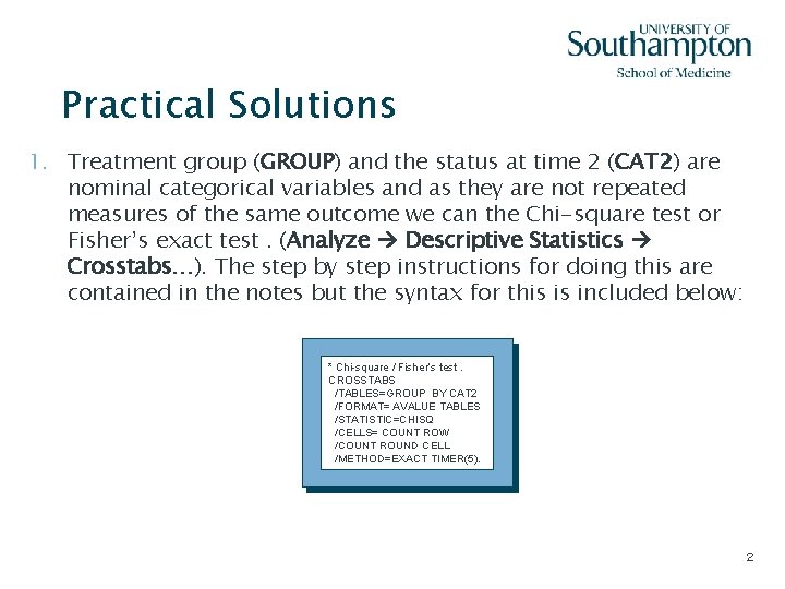
Practical Solutions 1. Treatment group (GROUP) and the status at time 2 (CAT 2) are nominal categorical variables and as they are not repeated measures of the same outcome we can the Chi-square test or Fisher’s exact test. (Analyze Descriptive Statistics Crosstabs…). The step by step instructions for doing this are contained in the notes but the syntax for this is included below: * Chi-square / Fisher’s test. CROSSTABS /TABLES=GROUP BY CAT 2 /FORMAT= AVALUE TABLES /STATISTIC=CHISQ /CELLS= COUNT ROW /COUNT ROUND CELL /METHOD=EXACT TIMER(5). 2

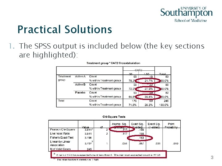
Practical Solutions 1. The SPSS output is included below (the key sections are highlighted): 3

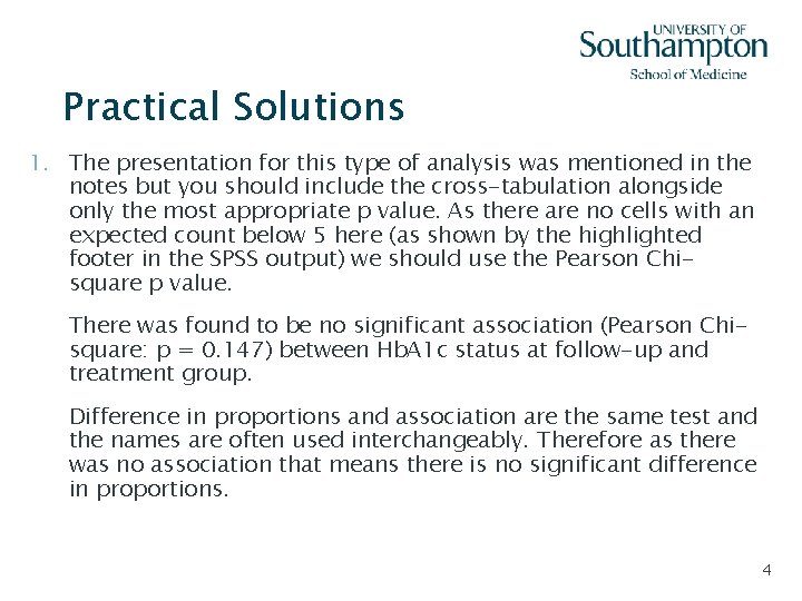
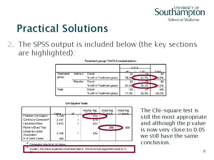
Practical Solutions 1. The presentation for this type of analysis was mentioned in the notes but you should include the cross-tabulation alongside only the most appropriate p value. As there are no cells with an expected count below 5 here (as shown by the highlighted footer in the SPSS output) we should use the Pearson Chisquare p value. There was found to be no significant association (Pearson Chisquare: p = 0. 147) between Hb. A 1 c status at follow-up and treatment group. Difference in proportions and association are the same test and the names are often used interchangeably. Therefore as there was no association that means there is no significant difference in proportions. 4

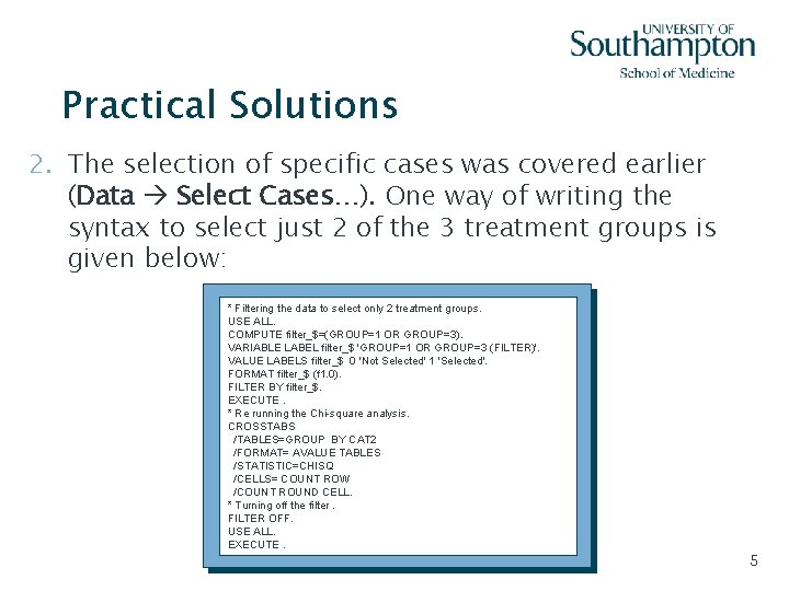
Practical Solutions 2. The selection of specific cases was covered earlier (Data Select Cases…). One way of writing the syntax to select just 2 of the 3 treatment groups is given below: * Filtering the data to select only 2 treatment groups. USE ALL. COMPUTE filter_$=(GROUP=1 OR GROUP=3). VARIABLE LABEL filter_$ 'GROUP=1 OR GROUP=3 (FILTER)'. VALUE LABELS filter_$ 0 'Not Selected' 1 'Selected'. FORMAT filter_$ (f 1. 0). FILTER BY filter_$. EXECUTE. * Re running the Chi-square analysis. CROSSTABS /TABLES=GROUP BY CAT 2 /FORMAT= AVALUE TABLES /STATISTIC=CHISQ /CELLS= COUNT ROW /COUNT ROUND CELL. * Turning off the filter. FILTER OFF. USE ALL. EXECUTE. 5

Practical Solutions 2. The SPSS output is included below (the key sections are highlighted): The Chi-square test is still the most appropriate and although the p value is now very close to 0. 05 we still have the same conclusion. 6

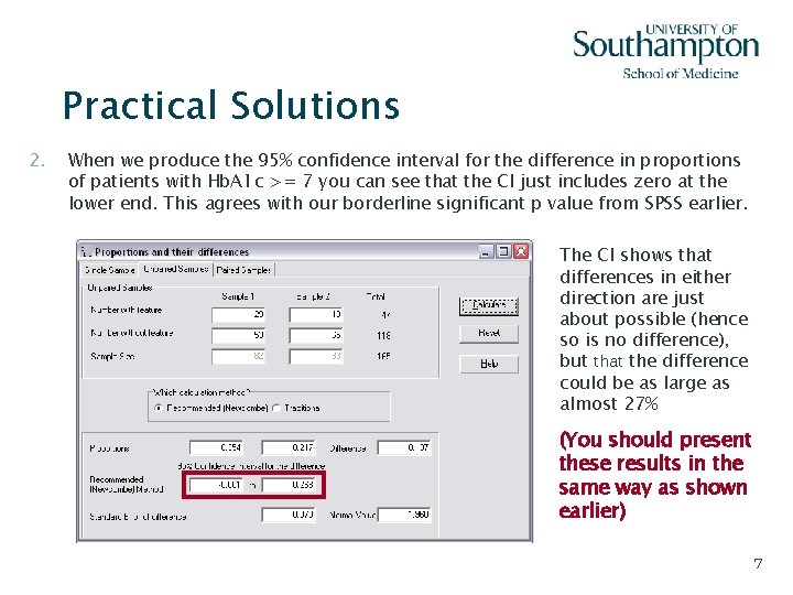
Practical Solutions 2. When we produce the 95% confidence interval for the difference in proportions of patients with Hb. A 1 c >= 7 you can see that the CI just includes zero at the lower end. This agrees with our borderline significant p value from SPSS earlier. The CI shows that differences in either direction are just about possible (hence so is no difference), but that the difference could be as large as almost 27% (You should present these results in the same way as shown earlier) 7

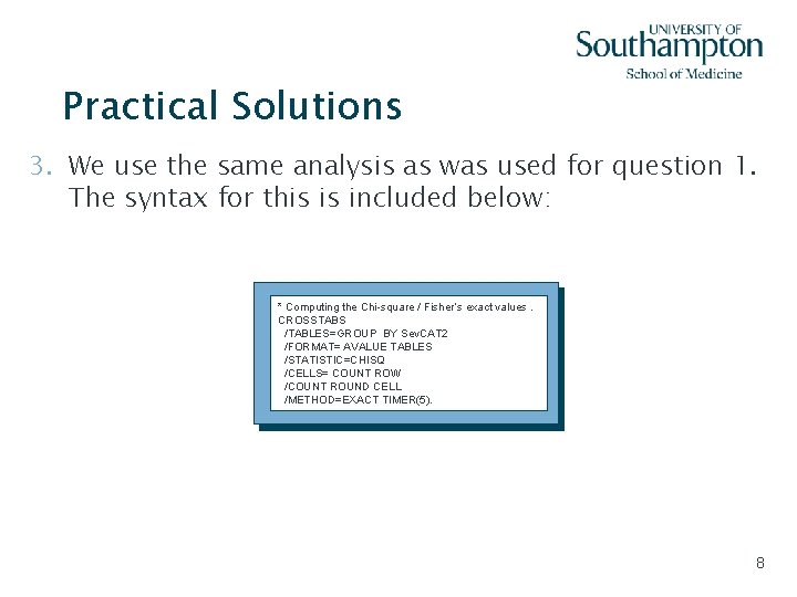
Practical Solutions 3. We use the same analysis as was used for question 1. The syntax for this is included below: * Computing the Chi-square / Fisher’s exact values. CROSSTABS /TABLES=GROUP BY Sev. CAT 2 /FORMAT= AVALUE TABLES /STATISTIC=CHISQ /CELLS= COUNT ROW /COUNT ROUND CELL /METHOD=EXACT TIMER(5). 8

Practical Solutions 3. The SPSS output is included below (the key sections are highlighted): 9

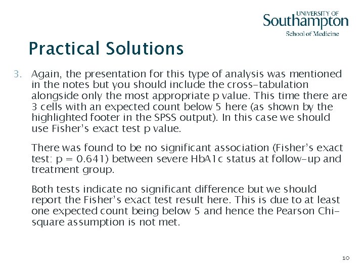
Practical Solutions 3. Again, the presentation for this type of analysis was mentioned in the notes but you should include the cross-tabulation alongside only the most appropriate p value. This time there are 3 cells with an expected count below 5 here (as shown by the highlighted footer in the SPSS output). In this case we should use Fisher’s exact test p value. There was found to be no significant association (Fisher’s exact test: p = 0. 641) between severe Hb. A 1 c status at follow-up and treatment group. Both tests indicate no significant difference but we should report the Fisher’s exact test result here. This is due to at least one expected count being below 5 and hence the Pearson Chisquare assumption is not met. 10

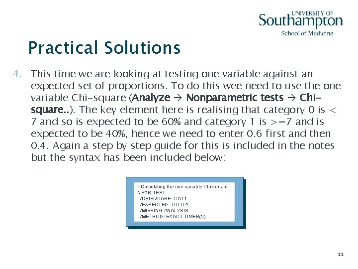
Practical Solutions 4. This time we are looking at testing one variable against an expected set of proportions. To do this wee need to use the one variable Chi-square (Analyze Nonparametric tests Chisquare. . ). The key element here is realising that category 0 is < 7 and so is expected to be 60% and category 1 is >=7 and is expected to be 40%, hence we need to enter 0. 6 first and then 0. 4. Again a step by step guide for this is included in the notes but the syntax has been included below: * Calculating the one variable Chi-square. NPAR TEST /CHISQUARE=CAT 1 /EXPECTED= 0. 6 0. 4 /MISSING ANALYSIS /METHOD=EXACT TIMER(5). 11

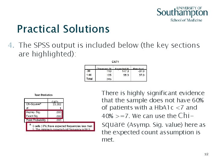
Practical Solutions 4. The SPSS output is included below (the key sections are highlighted): There is highly significant evidence that the sample does not have 60% of patients with a Hb. A 1 c <7 and 40% >=7. We can use the Chisquare (Asymp. Sig. value) here as the expected count assumption is met. 12

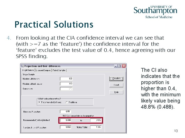
Practical Solutions 4. From looking at the CIA confidence interval we can see that (with >=7 as the ‘feature’) the confidence interval for the ‘feature’ excludes the test value of 0. 4, hence agreeing with our SPSS finding. The CI also indicates that the proportion is higher than 0. 4, with the minimum likely value being 48. 8% (0. 488). 13

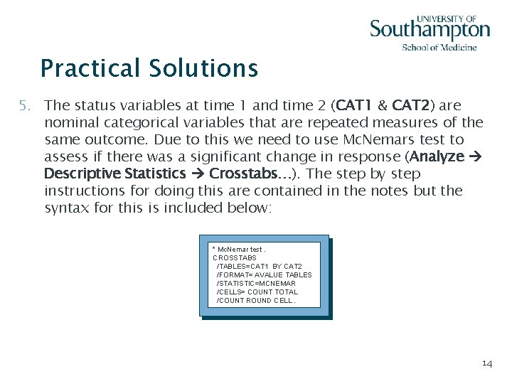
Practical Solutions 5. The status variables at time 1 and time 2 (CAT 1 & CAT 2) are nominal categorical variables that are repeated measures of the same outcome. Due to this we need to use Mc. Nemars test to assess if there was a significant change in response (Analyze Descriptive Statistics Crosstabs…). The step by step instructions for doing this are contained in the notes but the syntax for this is included below: * Mc. Nemar test. CROSSTABS /TABLES=CAT 1 BY CAT 2 /FORMAT= AVALUE TABLES /STATISTIC=MCNEMAR /CELLS= COUNT TOTAL /COUNT ROUND CELL. 14

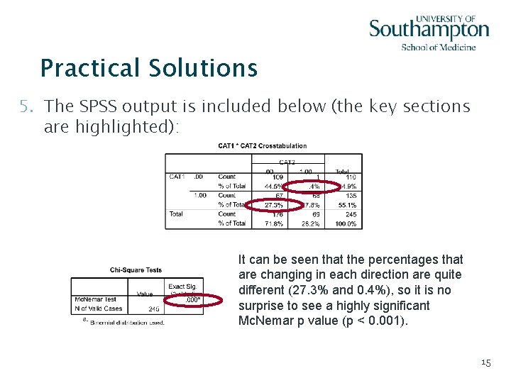
Practical Solutions 5. The SPSS output is included below (the key sections are highlighted): It can be seen that the percentages that are changing in each direction are quite different (27. 3% and 0. 4%), so it is no surprise to see a highly significant Mc. Nemar p value (p < 0. 001). 15

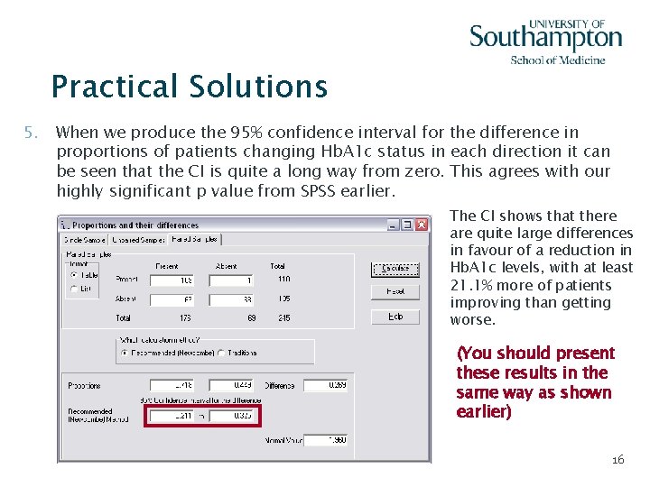
Practical Solutions 5. When we produce the 95% confidence interval for the difference in proportions of patients changing Hb. A 1 c status in each direction it can be seen that the CI is quite a long way from zero. This agrees with our highly significant p value from SPSS earlier. The CI shows that there are quite large differences in favour of a reduction in Hb. A 1 c levels, with at least 21. 1% more of patients improving than getting worse. (You should present these results in the same way as shown earlier) 16

Practical Solutions 5. Yet again the presentation for this type of analysis was mentioned in the notes but it should include the cross-tabulation, alongside the Mc. Nemar p value and a confidence interval for the difference in proportions changing in each direction. There was found to be a highly significant change in Hb. A 1 c control status (Mc. Nemar test: p < 0. 001) between the two measurements in favour of improving control or a lowering of Hb. A 1 c levels (Difference 26. 9%, 95% CI: 21. 1% to 32. 5%). 17

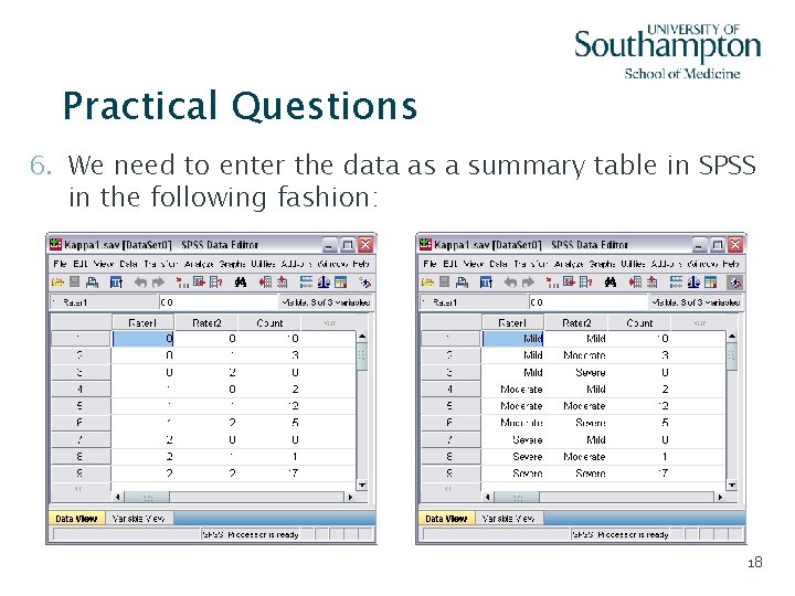
Practical Questions 6. We need to enter the data as a summary table in SPSS in the following fashion: 18

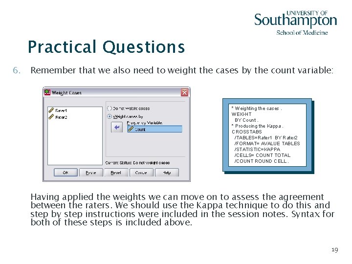
Practical Questions 6. Remember that we also need to weight the cases by the count variable: * Weighting the cases. WEIGHT BY Count. * Producing the Kappa. CROSSTABS /TABLES=Rater 1 BY Rater 2 /FORMAT= AVALUE TABLES /STATISTIC=KAPPA /CELLS= COUNT TOTAL /COUNT ROUND CELL. Having applied the weights we can move on to assess the agreement between the raters. We should use the Kappa technique to do this and step by step instructions were included in the session notes. Syntax for both of these steps is included above. 19

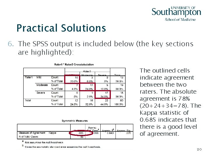
Practical Solutions 6. The SPSS output is included below (the key sections are highlighted): The outlined cells indicate agreement between the two raters. The absolute agreement is 78% (20+24+34=78). The Kappa statistic of 0. 685 indicates that there is a good level of agreement. 20

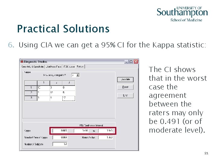
Practical Solutions 6. Using CIA we can get a 95% CI for the Kappa statistic: The CI shows that in the worst case the agreement between the raters may only be 0. 491 (or of moderate level). 21