Practical Aspects of Quantum Coin Flipping Anna Pappa

Practical Aspects of Quantum Coin Flipping Anna Pappa Presentation at ACAC 2012

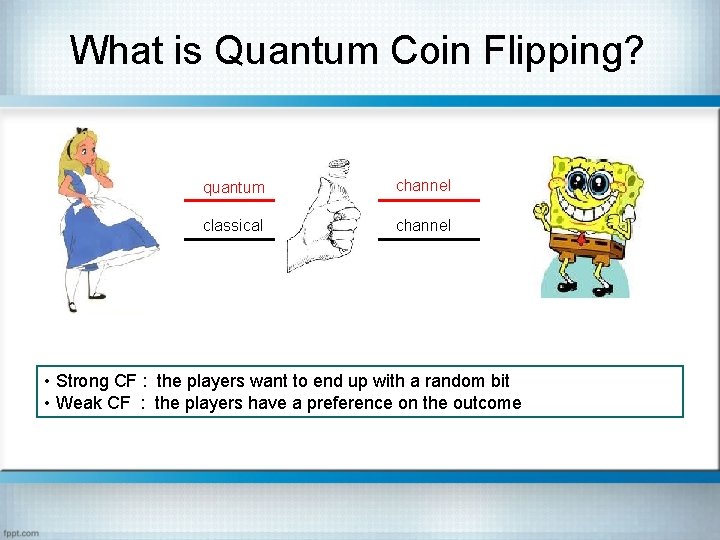
What is Quantum Coin Flipping? quantum channel classical channel • Strong CF : the players want to end up with a random bit • Weak CF : the players have a preference on the outcome

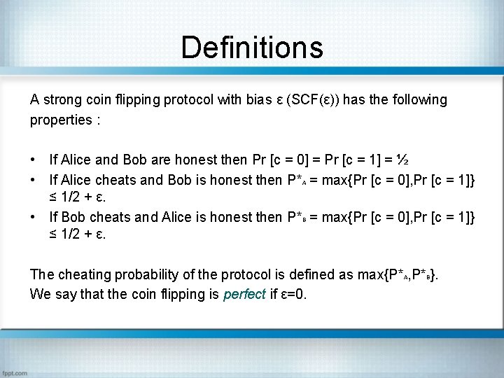
Definitions A strong coin flipping protocol with bias ε (SCF(ε)) has the following properties : • If Alice and Bob are honest then Pr [c = 0] = Pr [c = 1] = ½ • If Alice cheats and Bob is honest then P* = max{Pr [c = 0], Pr [c = 1]} ≤ 1/2 + ε. • If Bob cheats and Alice is honest then P* = max{Pr [c = 0], Pr [c = 1]} ≤ 1/2 + ε. Α Β The cheating probability of the protocol is defined as max{P* , P* }. We say that the coin flipping is perfect if ε=0. Α B

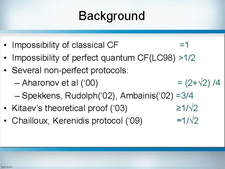
Background • Impossibility of classical CF =1 • Impossibility of perfect quantum CF(LC 98) >1/2 • Several non-perfect protocols: – Aharonov et al (‘ 00) = (2+√ 2) /4 – Spekkens, Rudolph(‘ 02), Ambainis(’ 02) =3/4 • Kitaev’s theoretical proof (‘ 03) ≥ 1/√ 2 • Chailloux, Kerenidis protocol (‘ 09) ≈1/√ 2

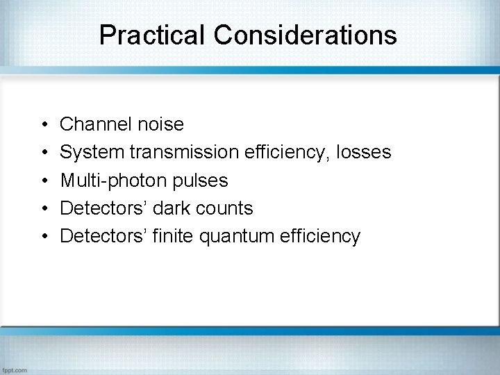
Practical Considerations • • • Channel noise System transmission efficiency, losses Multi-photon pulses Detectors’ dark counts Detectors’ finite quantum efficiency

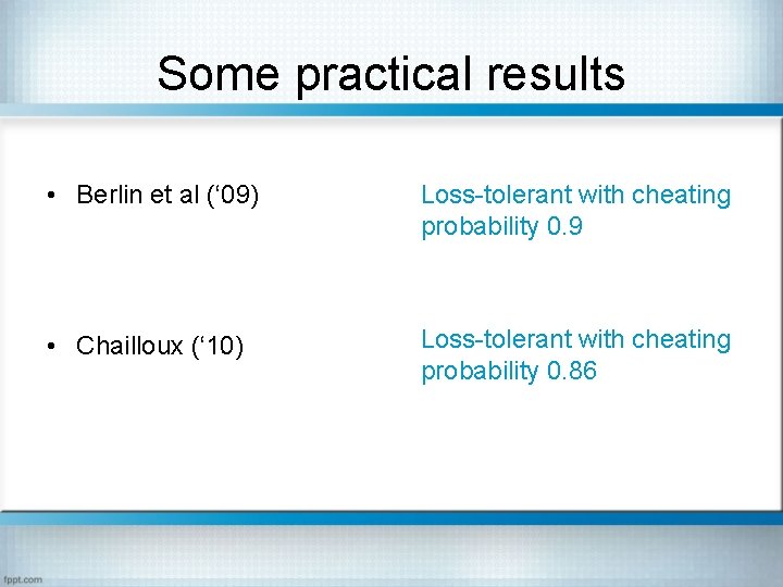
Some practical results • Berlin et al (‘ 09) Loss-tolerant with cheating probability 0. 9 • Chailloux (‘ 10) Loss-tolerant with cheating probability 0. 86

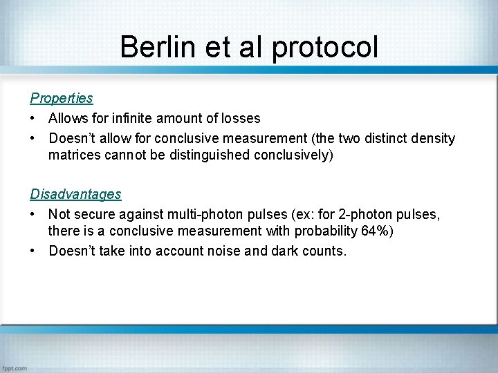
Berlin et al protocol Properties • Allows for infinite amount of losses • Doesn’t allow for conclusive measurement (the two distinct density matrices cannot be distinguished conclusively) Disadvantages • Not secure against multi-photon pulses (ex: for 2 -photon pulses, there is a conclusive measurement with probability 64%) • Doesn’t take into account noise and dark counts.

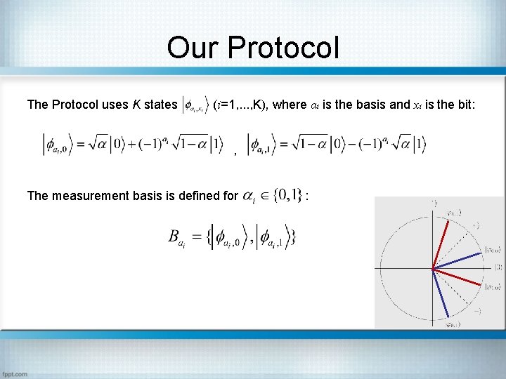
Our Protocol The Protocol uses K states (i=1, . . . , K), where αi is the basis and xi is the bit: , The measurement basis is defined for :

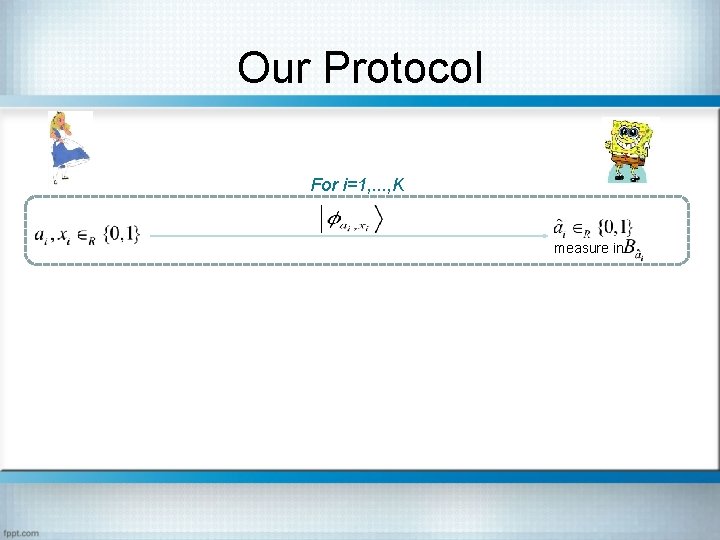
Our Protocol For i=1, . . . , K measure in

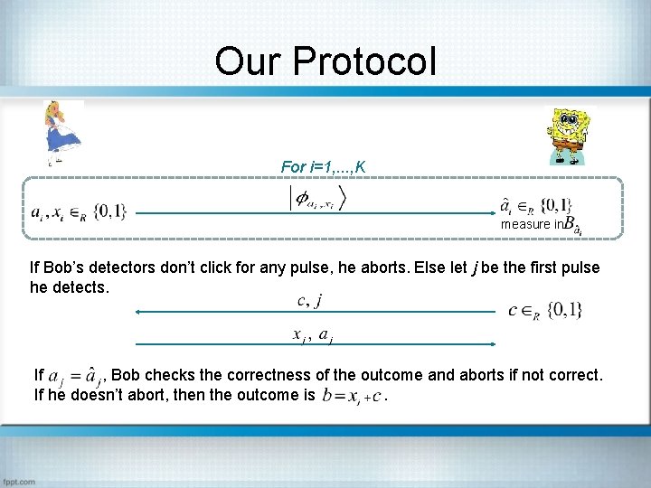
Our Protocol For i=1, . . . , K measure in If Bob’s detectors don’t click for any pulse, he aborts. Else let j be the first pulse he detects. If , Bob checks the correctness of the outcome and aborts if not correct. If he doesn’t abort, then the outcome is.

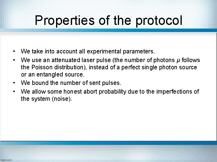
Properties of the protocol • We take into account all experimental parameters. • We use an attenuated laser pulse (the number of photons μ follows the Poisson distribution), instead of a perfect single photon source or an entangled source. • We bound the number of sent pulses. • We allow some honest abort probability due to the imperfections of the system (noise).

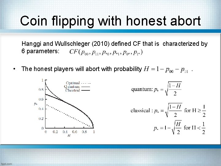
Coin flipping with honest abort Hanggi and Wullschleger (2010) defined CF that is characterized by 6 parameters: • The honest players will abort with probability .

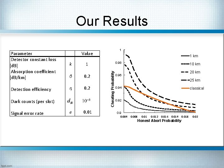
Our Results k 1 β 0. 2 Detection efficiency η 0. 2 Dark counts (per slot) Signal error rate 1 Value e 0. 01 1 km 0. 98 Cheating Probability Parameter Detector constant loss [d. B] Absorption coefficient [d. B/km] 10 km 20 km 0. 96 25 km 0. 94 classical 0. 92 0. 9 0. 006 0. 008 0. 012 0. 014 0. 016 Honest Abort Probability 0. 018 0. 02

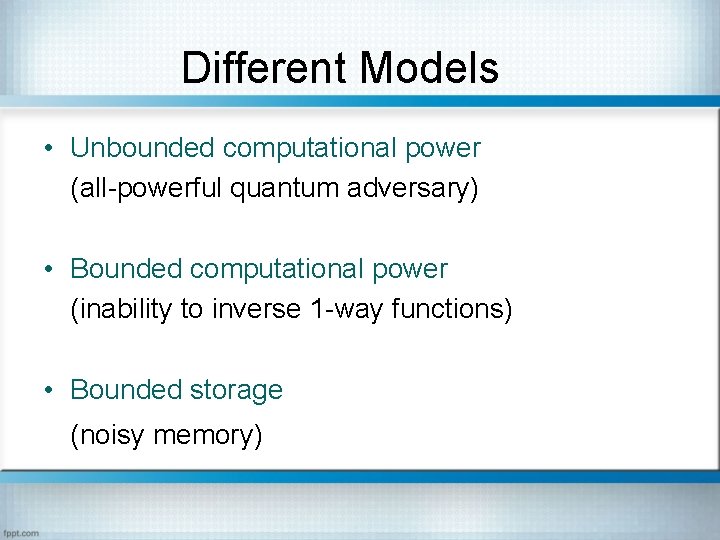
Different Models • Unbounded computational power (all-powerful quantum adversary) • Bounded computational power (inability to inverse 1 -way functions) • Bounded storage (noisy memory)

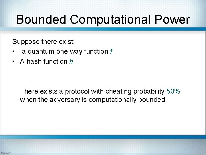
Bounded Computational Power Suppose there exist: • a quantum one-way function f • A hash function h There exists a protocol with cheating probability 50% when the adversary is computationally bounded.

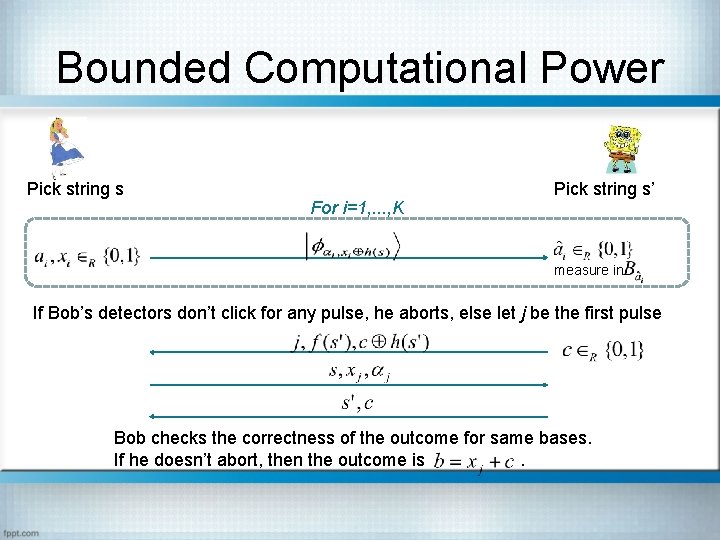
Bounded Computational Power Pick string s For i=1, . . . , K Pick string s’ measure in If Bob’s detectors don’t click for any pulse, he aborts, else let j be the first pulse Bob checks the correctness of the outcome for same bases. If he doesn’t abort, then the outcome is.

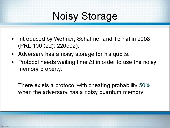
Noisy Storage • Introduced by Wehner, Schaffner and Terhal in 2008 (PRL 100 (22): 220502). • Adversary has a noisy storage for his qubits. • Protocol needs waiting time Δt in order to use the noisy memory property. There exists a protocol with cheating probability 50% when the adversary has a noisy quantum memory.

Implementations 1. G. Molina-Terriza, A. Vaziri, R. Ursin and A. Zeilinger (2005) 2. A. T. Nguyen, J. Frison, K. Phan Huy and S. Massar (2008) 3. G. Berlin, G. Brassard, F. Bussières, N. Godbout, J. A. Slater and W. Tittel (2009)

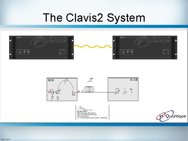
The Clavis 2 System