Perfect Competition 2012 Cengage Learning All Rights Reserved

Perfect Competition © 2012 Cengage Learning. All Rights Reserved. May not be copied, scanned, or duplicated, in whole or in part, except for use as permitted in a license distributed with a certain product or service or otherwise on a password-protected website for classroom use. 1

Introduction to Perfect Competition • Market structure – Number of suppliers – Ease of entry into the market – Similar products • A firm’s decisions – How much to produce; what price to charge – Depend on the structure of the market © 2012 Cengage Learning. All Rights Reserved. May not be copied, scanned, or duplicated, in whole or in part, except for use as permitted in a license distributed with a certain product or service or otherwise on a password-protected website for classroom use. 2

Perfectly Competitive Market • Perfect competition – Many buyers and sellers – Commodity; standardized product – Fully informed buyers and sellers – No barriers to entry • Individual buyer or seller – No control over price – Price takers © 2012 Cengage Learning. All Rights Reserved. May not be copied, scanned, or duplicated, in whole or in part, except for use as permitted in a license distributed with a certain product or service or otherwise on a password-protected website for classroom use. 3

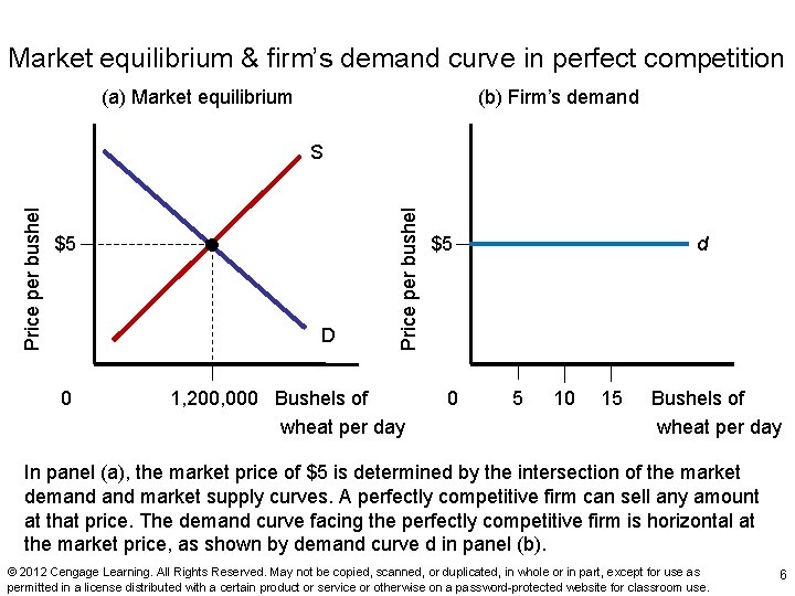
Demand under Perfect Competition • Market price – Determined by supply and demand • Demand curve facing one supplier – Horizontal line at the market price – Perfectly elastic © 2012 Cengage Learning. All Rights Reserved. May not be copied, scanned, or duplicated, in whole or in part, except for use as permitted in a license distributed with a certain product or service or otherwise on a password-protected website for classroom use. 4

Demand under Perfect Competition • Price taker – Firm that faces a given market price • Its quantity supplied has no effect on that price – Perfectly competitive firm that decides to produce • Must accept, or “take, ” the market price © 2012 Cengage Learning. All Rights Reserved. May not be copied, scanned, or duplicated, in whole or in part, except for use as permitted in a license distributed with a certain product or service or otherwise on a password-protected website for classroom use. 5

Exhibit 1 Market equilibrium & firm’s demand curve in perfect competition (b) Firm’s demand (a) Market equilibrium $5 D 0 Price per bushel S 1, 200, 000 Bushels of wheat per day $5 0 d 5 10 15 Bushels of wheat per day In panel (a), the market price of $5 is determined by the intersection of the market demand market supply curves. A perfectly competitive firm can sell any amount at that price. The demand curve facing the perfectly competitive firm is horizontal at the market price, as shown by demand curve d in panel (b). © 2012 Cengage Learning. All Rights Reserved. May not be copied, scanned, or duplicated, in whole or in part, except for use as permitted in a license distributed with a certain product or service or otherwise on a password-protected website for classroom use. 6

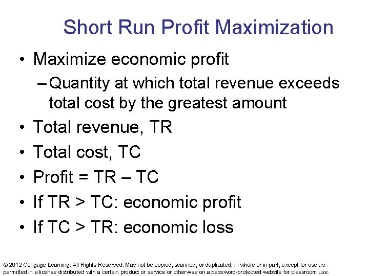
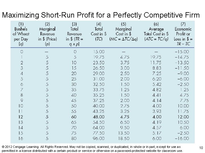
Short Run Profit Maximization • Maximize economic profit – Quantity at which total revenue exceeds total cost by the greatest amount • Total revenue, TR • • Total cost, TC Profit = TR – TC If TR > TC: economic profit If TC > TR: economic loss © 2012 Cengage Learning. All Rights Reserved. May not be copied, scanned, or duplicated, in whole or in part, except for use as permitted in a license distributed with a certain product or service or otherwise on a password-protected website for classroom use. 7

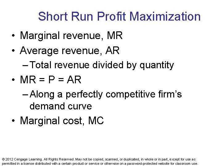
Short Run Profit Maximization • Marginal revenue, MR • Average revenue, AR – Total revenue divided by quantity • MR = P = AR – Along a perfectly competitive firm’s demand curve • Marginal cost, MC © 2012 Cengage Learning. All Rights Reserved. May not be copied, scanned, or duplicated, in whole or in part, except for use as permitted in a license distributed with a certain product or service or otherwise on a password-protected website for classroom use. 8

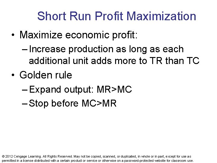
Short Run Profit Maximization • Maximize economic profit: – Increase production as long as each additional unit adds more to TR than TC • Golden rule – Expand output: MR>MC – Stop before MC>MR © 2012 Cengage Learning. All Rights Reserved. May not be copied, scanned, or duplicated, in whole or in part, except for use as permitted in a license distributed with a certain product or service or otherwise on a password-protected website for classroom use. 9

Exhibit 2 Maximizing Short-Run Profit for a Perfectly Competitive Firm © 2012 Cengage Learning. All Rights Reserved. May not be copied, scanned, or duplicated, in whole or in part, except for use as permitted in a license distributed with a certain product or service or otherwise on a password-protected website for classroom use. 10

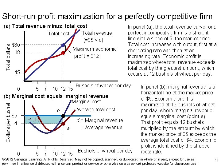
Exhibit 3 Short-run profit maximization for a perfectly competitive firm (a) Total revenue minus total cost Total revenue (=$5 × q) Total dollars Total cost $60 Maximum economic profit = $12 48 15 0 5 7 10 12 15 In panel (a), the total revenue curve for a perfectly competitive firm is a straight line with a slope of 5, the market price. Total cost increases with output, first at a decreasing rate and then at an increasing rate. Economic profit is maximized where total revenue exceeds total cost by the greatest amount, which occurs at 12 bushels of wheat per day. Bushels of wheat per day Dollars per bushel (b) Marginal cost equals marginal revenue Marginal cost Average total cost e $5 Profit 4 a 0 5 7 10 12 15 d = Marginal revenue = Average revenue Bushels of wheat per day In panel (b), marginal revenue is a horizontal line at the market price of $5. Economic profit is maximized at 12 bushels of wheat per day, where marginal revenue equals marginal cost (point e). That profit equals 12 bushels multiplied by the amount by which the market price of $5 exceeds the average total cost of $4. Economic profit is identified by the shaded rectangle. © 2012 Cengage Learning. All Rights Reserved. May not be copied, scanned, or duplicated, in whole or in part, except for use as permitted in a license distributed with a certain product or service or otherwise on a password-protected website for classroom use. 11

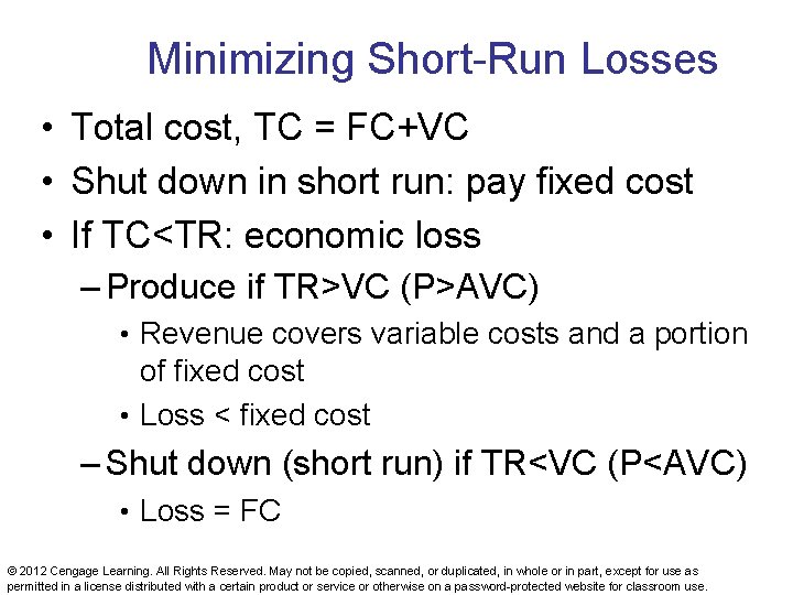
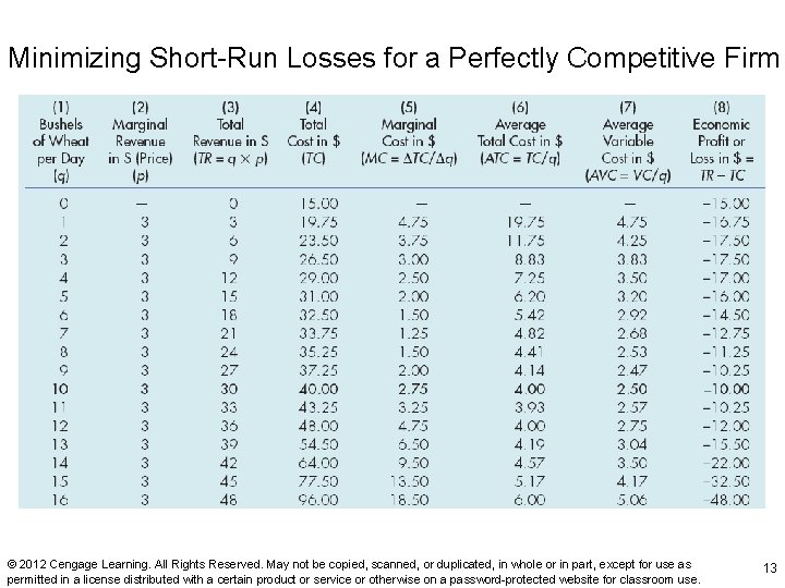
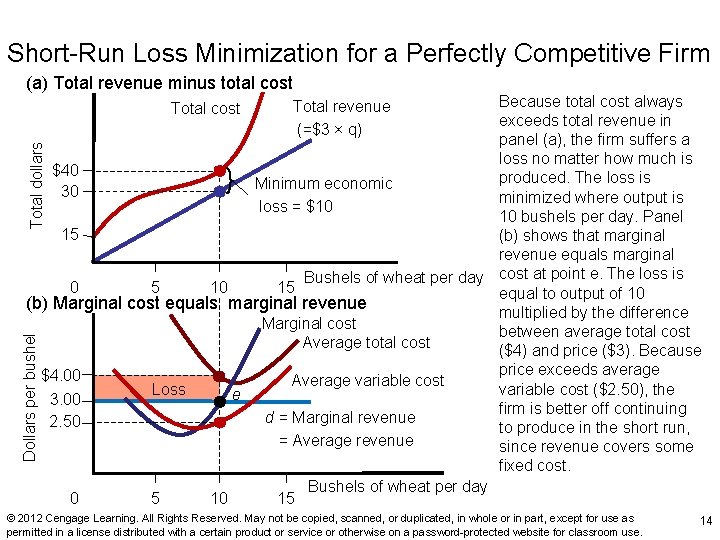
Minimizing Short-Run Losses • Total cost, TC = FC+VC • Shut down in short run: pay fixed cost • If TC<TR: economic loss – Produce if TR>VC (P>AVC) • Revenue covers variable costs and a portion of fixed cost • Loss < fixed cost – Shut down (short run) if TR<VC (P<AVC) • Loss = FC © 2012 Cengage Learning. All Rights Reserved. May not be copied, scanned, or duplicated, in whole or in part, except for use as permitted in a license distributed with a certain product or service or otherwise on a password-protected website for classroom use. 12

Exhibit 4 Minimizing Short-Run Losses for a Perfectly Competitive Firm © 2012 Cengage Learning. All Rights Reserved. May not be copied, scanned, or duplicated, in whole or in part, except for use as permitted in a license distributed with a certain product or service or otherwise on a password-protected website for classroom use. 13

Exhibit 5 Short-Run Loss Minimization for a Perfectly Competitive Firm (a) Total revenue minus total cost Because total cost always exceeds total revenue in panel (a), the firm suffers a loss no matter how much is $40 produced. The loss is Minimum economic 30 minimized where output is loss = $10 10 bushels per day. Panel 15 (b) shows that marginal revenue equals marginal Bushels of wheat per day cost at point e. The loss is 0 5 10 15 equal to output of 10 (b) Marginal cost equals marginal revenue multiplied by the difference Marginal cost between average total cost Average total cost ($4) and price ($3). Because price exceeds average $4. 00 Average variable cost ($2. 50), the Loss e 3. 00 firm is better off continuing d = Marginal revenue 2. 50 to produce in the short run, = Average revenue since revenue covers some fixed cost. Bushels of wheat per day 0 5 10 15 Total revenue (=$3 × q) Dollars per bushel Total dollars Total cost © 2012 Cengage Learning. All Rights Reserved. May not be copied, scanned, or duplicated, in whole or in part, except for use as permitted in a license distributed with a certain product or service or otherwise on a password-protected website for classroom use. 14

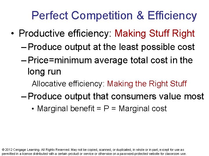
Perfect Competition & Efficiency • Productive efficiency: Making Stuff Right – Produce output at the least possible cost – Price=minimum average total cost in the long run Allocative efficiency: Making the Right Stuff – Produce output that consumers value most • Marginal benefit = P = Marginal cost © 2012 Cengage Learning. All Rights Reserved. May not be copied, scanned, or duplicated, in whole or in part, except for use as permitted in a license distributed with a certain product or service or otherwise on a password-protected website for classroom use. 15

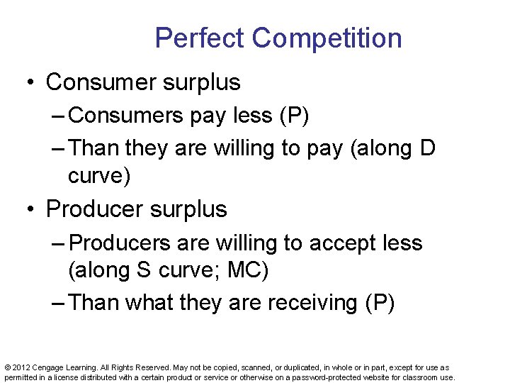
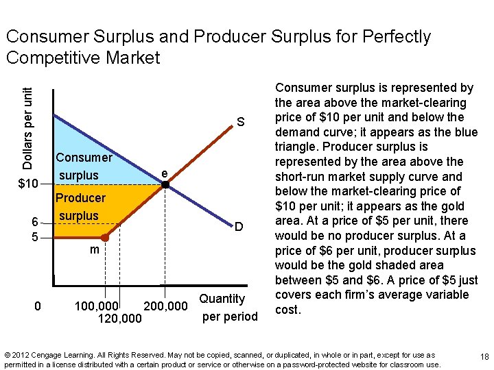
Perfect Competition • Consumer surplus – Consumers pay less (P) – Than they are willing to pay (along D curve) • Producer surplus – Producers are willing to accept less (along S curve; MC) – Than what they are receiving (P) © 2012 Cengage Learning. All Rights Reserved. May not be copied, scanned, or duplicated, in whole or in part, except for use as permitted in a license distributed with a certain product or service or otherwise on a password-protected website for classroom use. 16

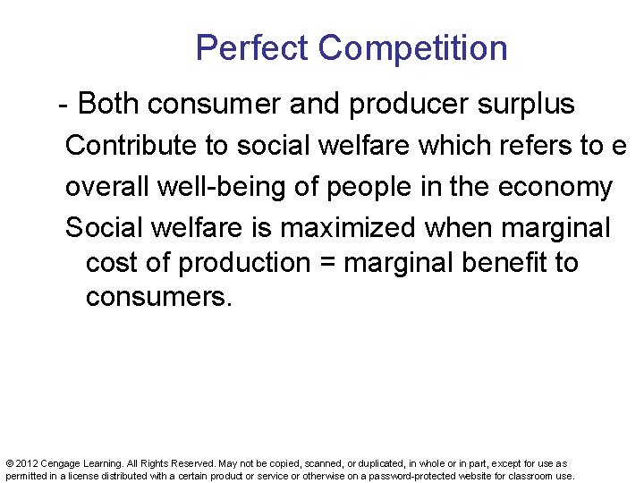
Perfect Competition - Both consumer and producer surplus Contribute to social welfare which refers to e overall well-being of people in the economy Social welfare is maximized when marginal cost of production = marginal benefit to consumers. © 2012 Cengage Learning. All Rights Reserved. May not be copied, scanned, or duplicated, in whole or in part, except for use as permitted in a license distributed with a certain product or service or otherwise on a password-protected website for classroom use. 17

Exhibit 13 Dollars per unit Consumer Surplus and Producer Surplus for Perfectly Competitive Market S $10 6 5 0 Consumer surplus e Producer surplus D m 100, 000 200, 000 120, 000 Quantity period Consumer surplus is represented by the area above the market-clearing price of $10 per unit and below the demand curve; it appears as the blue triangle. Producer surplus is represented by the area above the short-run market supply curve and below the market-clearing price of $10 per unit; it appears as the gold area. At a price of $5 per unit, there would be no producer surplus. At a price of $6 per unit, producer surplus would be the gold shaded area between $5 and $6. A price of $5 just covers each firm’s average variable cost. © 2012 Cengage Learning. All Rights Reserved. May not be copied, scanned, or duplicated, in whole or in part, except for use as permitted in a license distributed with a certain product or service or otherwise on a password-protected website for classroom use. 18