17 2012 Cengage Learning All Rights Reserved May

17 © 2012 Cengage Learning. All Rights Reserved. May not be copied, scanned, or duplicated, in whole or in part, except for use as permitted in a license distributed with a certain product or service or otherwise on a password-protected website for classroom use. 1

Active Policy vs. Passive Policy • Active approach – Economy - relatively unstable • Fluctuations – from private sector – Government intervention – Discretionary fiscal or monetary policy • Passive approach – Economy – relatively stable – Natural market forces – Automatic stabilizers © 2012 Cengage Learning. All Rights Reserved. May not be copied, scanned, or duplicated, in whole or in part, except for use as permitted in a license distributed with a certain product or service or otherwise on a password-protected website for classroom use. 2

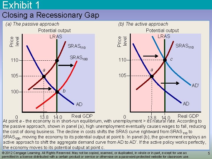
Closing a Recessionary Gap • Passive approach – Self-correcting forces of the economy – Wages and prices are flexible enough – High unemployment – decrease in wages and production costs – Increase SRAS • Potential output – Automatic stabilizers – No discretionary policy © 2012 Cengage Learning. All Rights Reserved. May not be copied, scanned, or duplicated, in whole or in part, except for use as permitted in a license distributed with a certain product or service or otherwise on a password-protected website for classroom use. 3

Closing a Recessionary Gap • Active approach – Prices and wages are not flexible – Unemployment above natural rate • Market forces may be too slow to respond – Stimulate aggregate demand • Fiscal policy • Monetary policy – Increase in price level © 2012 Cengage Learning. All Rights Reserved. May not be copied, scanned, or duplicated, in whole or in part, except for use as permitted in a license distributed with a certain product or service or otherwise on a password-protected website for classroom use. 4

Exhibit 1 Closing a Recessionary Gap (b) The active approach Potential output LRAS SRAS 110 SRAS 100 110 Price level (a) The passive approach Potential output LRAS SRAS 110 c 110 a a 105 AD’ b 100 AD AD 0 13. 8 14. 0 Real GDP At point a - the economy is in short-run equilibrium, with unemployment > its natural rate. According to the passive approach, shown in panel (a), high unemployment eventually causes wages to fall, reducing the cost of doing business. The decline in costs shifts the SRAS curve rightward from SRAS 110 to SRAS 100, moving the economy to its potential output at point b. In panel (b), the government employs an active approach to shift the aggregate demand curve from AD to AD’. If the active policy works perfectly, the economy moves to its potential output at point c. © 2012 Cengage Learning. All Rights Reserved. May not be copied, scanned, or duplicated, in whole or in part, except for use as permitted in a license distributed with a certain product or service or otherwise on a password-protected website for classroom use. 5

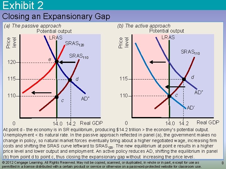
Closing an Expansionary Gap • Passive approach – Self-correcting forces • Negotiate higher wages • Higher production costs – Decrease SRAS • Potential output • Higher price level – Automatic stabilizers – No discretionary policy © 2012 Cengage Learning. All Rights Reserved. May not be copied, scanned, or duplicated, in whole or in part, except for use as permitted in a license distributed with a certain product or service or otherwise on a password-protected website for classroom use. 6

Closing an Expansionary Gap • Active approach – Prices and wages are not flexible – Decrease aggregate demand • Fiscal policy • Monetary policy – Lower price level © 2012 Cengage Learning. All Rights Reserved. May not be copied, scanned, or duplicated, in whole or in part, except for use as permitted in a license distributed with a certain product or service or otherwise on a password-protected website for classroom use. 7

Exhibit 2 Closing an Expansionary Gap 120 SRAS 110 e 115 110 (b) The active approach Potential output LRAS Price level (a) The passive approach Potential output LRAS SRAS 120 c d 115 d AD” 110 AD” c AD’ 0 14. 2 Real GDP At point d - the economy is in SR equilibrium, producing $14. 2 trillion > the economy’s potential output. Unemployment < its natural rate. In the passive approach reflected in panel (a), the government makes no change in policy, so natural market forces eventually bring about a higher negotiated wage, increasing firm costs and shifting the SRAS curve leftward to SRAS 120. The new equilibrium at point e results in a higher price level and lower output and employment. An active policy reduces AD, shifting the equilibrium in panel (b) from point d to point c, thus closing the expansionary gap without increasing the price level. © 2012 Cengage Learning. All Rights Reserved. May not be copied, scanned, or duplicated, in whole or in part, except for use as permitted in a license distributed with a certain product or service or otherwise on a password-protected website for classroom use. 8

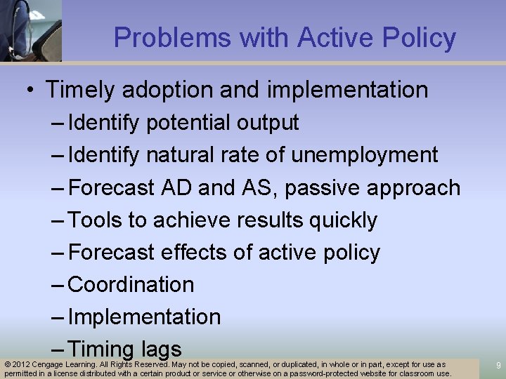
Problems with Active Policy • Timely adoption and implementation – Identify potential output – Identify natural rate of unemployment – Forecast AD and AS, passive approach – Tools to achieve results quickly – Forecast effects of active policy – Coordination – Implementation – Timing lags © 2012 Cengage Learning. All Rights Reserved. May not be copied, scanned, or duplicated, in whole or in part, except for use as permitted in a license distributed with a certain product or service or otherwise on a password-protected website for classroom use. 9

The Problem of Lags • Recognition lag – Time needed to identify a macroeconomic problem and assess its seriousness • Decision-making lag – Time needed to decide what to do once a macroeconomic problem has been identified © 2012 Cengage Learning. All Rights Reserved. May not be copied, scanned, or duplicated, in whole or in part, except for use as permitted in a license distributed with a certain product or service or otherwise on a password-protected website for classroom use. 10

The Problem of Lags • Implementation lag – Time needed to introduce a change in monetary or fiscal policy – Longer for fiscal policy • Effectiveness lag – Time needed for changes in monetary or fiscal policy to affect the economy © 2012 Cengage Learning. All Rights Reserved. May not be copied, scanned, or duplicated, in whole or in part, except for use as permitted in a license distributed with a certain product or service or otherwise on a password-protected website for classroom use. 11

The Role of Expectations • Rational expectations – People form expectations based on all available information – Including the likely future actions of government policy makers © 2012 Cengage Learning. All Rights Reserved. May not be copied, scanned, or duplicated, in whole or in part, except for use as permitted in a license distributed with a certain product or service or otherwise on a password-protected website for classroom use. 12

The Role of Expectations • Potential output; natural rate – Fed policy pronouncements • Sustain potential output • Stable price level – Fed actions: unexpected expansionary policy • Higher equilibrium output • Higher price level © 2012 Cengage Learning. All Rights Reserved. May not be copied, scanned, or duplicated, in whole or in part, except for use as permitted in a license distributed with a certain product or service or otherwise on a password-protected website for classroom use. 13

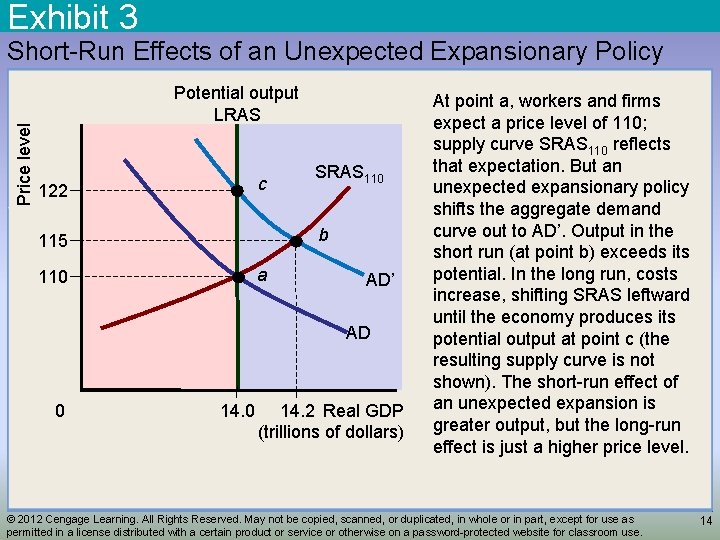
Exhibit 3 Price level Short-Run Effects of an Unexpected Expansionary Policy Potential output LRAS c 122 SRAS 110 b 115 a 110 AD’ AD 0 14. 2 Real GDP (trillions of dollars) At point a, workers and firms expect a price level of 110; supply curve SRAS 110 reflects that expectation. But an unexpected expansionary policy shifts the aggregate demand curve out to AD’. Output in the short run (at point b) exceeds its potential. In the long run, costs increase, shifting SRAS leftward until the economy produces its potential output at point c (the resulting supply curve is not shown). The short-run effect of an unexpected expansion is greater output, but the long-run effect is just a higher price level. © 2012 Cengage Learning. All Rights Reserved. May not be copied, scanned, or duplicated, in whole or in part, except for use as permitted in a license distributed with a certain product or service or otherwise on a password-protected website for classroom use. 14

The Role of Expectations • Time-inconsistency problem – When policy makers have an incentive to announce one policy • To influence expectations – But then pursue a different policy • Once those expectations have been formed and acted on © 2012 Cengage Learning. All Rights Reserved. May not be copied, scanned, or duplicated, in whole or in part, except for use as permitted in a license distributed with a certain product or service or otherwise on a password-protected website for classroom use. 15

Anticipating Policy • Potential output; High price level – Fed policy pronouncements • Sustain potential output & stable price level – Firms – don’t trust Fed • Expect higher price level – Fed actions: expected expansionary policy • Potential output • Higher price level © 2012 Cengage Learning. All Rights Reserved. May not be copied, scanned, or duplicated, in whole or in part, except for use as permitted in a license distributed with a certain product or service or otherwise on a password-protected website for classroom use. 16

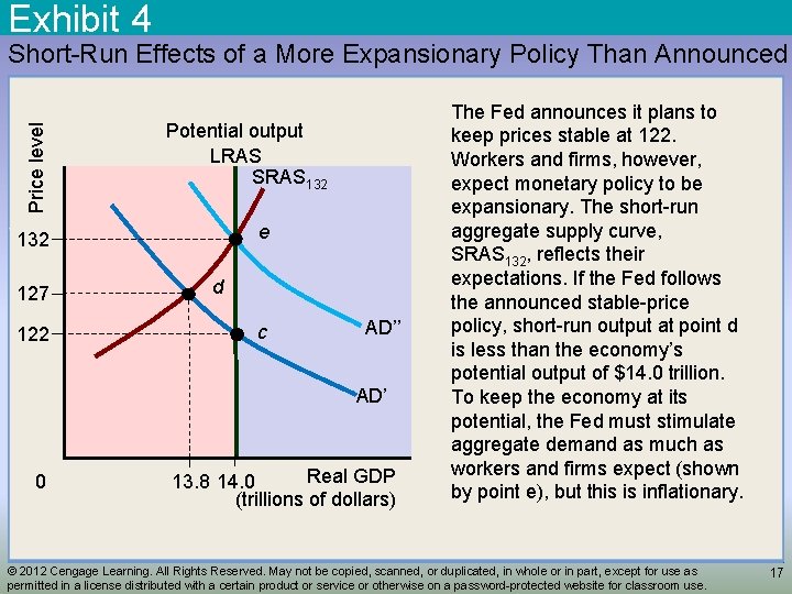
Exhibit 4 Price level Short-Run Effects of a More Expansionary Policy Than Announced Potential output LRAS SRAS 132 e 132 127 122 d c AD’’ AD’ 0 Real GDP 13. 8 14. 0 (trillions of dollars) The Fed announces it plans to keep prices stable at 122. Workers and firms, however, expect monetary policy to be expansionary. The short-run aggregate supply curve, SRAS 132, reflects their expectations. If the Fed follows the announced stable-price policy, short-run output at point d is less than the economy’s potential output of $14. 0 trillion. To keep the economy at its potential, the Fed must stimulate aggregate demand as much as workers and firms expect (shown by point e), but this is inflationary. © 2012 Cengage Learning. All Rights Reserved. May not be copied, scanned, or duplicated, in whole or in part, except for use as permitted in a license distributed with a certain product or service or otherwise on a password-protected website for classroom use. 17

Anticipating Policy • If the economy is already producing its potential – A fully anticipated expansionary policy • Has no effect on output or employment, not even in the short run. – Only unanticipated expansionary policy • Can temporarily push output beyond its potential. © 2012 Cengage Learning. All Rights Reserved. May not be copied, scanned, or duplicated, in whole or in part, except for use as permitted in a license distributed with a certain product or service or otherwise on a password-protected website for classroom use. 18

Policy Credibility • Economy: potential output – Unexpected expansionary policy • Temporary increase output, employment • Costs – Inflation in the long term – Credibility loss • Hyperinflation – Anti-inflation policy: cold turkey • Announce and execute tough measures © 2012 Cengage Learning. All Rights Reserved. May not be copied, scanned, or duplicated, in whole or in part, except for use as permitted in a license distributed with a certain product or service or otherwise on a password-protected website for classroom use. 19

Policy Rules vs. Discretion • Active approach – Economy is unstable – Needs discretionary policy to cut cyclical unemployment when it arises • Passive approach – Economy is stable enough – Discretionary policy • Unnecessary • May worsen economic fluctuations © 2012 Cengage Learning. All Rights Reserved. May not be copied, scanned, or duplicated, in whole or in part, except for use as permitted in a license distributed with a certain product or service or otherwise on a password-protected website for classroom use. 20

Policy Rules vs. Discretion • Passive approach – Fiscal policy - automatic stabilizers • Unemployment insurance • Progressive income tax, Transfer payments – Monetary policy • Allow the money supply to grow at a predetermined rate • Maintain interest rates at some predetermined level • Keep inflation below a certain rate © 2012 Cengage Learning. All Rights Reserved. May not be copied, scanned, or duplicated, in whole or in part, except for use as permitted in a license distributed with a certain product or service or otherwise on a password-protected website for classroom use. 21

Policy Rules vs. Discretion • Limitations on discretion – Complex interactions among economic aggregates – Lags • Rules and rational expectations – Fully anticipated monetary policy • No effect on output • Change price level © 2012 Cengage Learning. All Rights Reserved. May not be copied, scanned, or duplicated, in whole or in part, except for use as permitted in a license distributed with a certain product or service or otherwise on a password-protected website for classroom use. 22

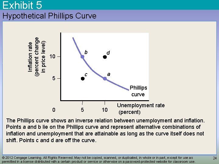
The Phillips Curve • Inverse relationship – Unemployment rate – Rate of change in nominal wages (inflation) • Phillips curve – A curve showing possible combinations of the inflation rate and the unemployment rate © 2012 Cengage Learning. All Rights Reserved. May not be copied, scanned, or duplicated, in whole or in part, except for use as permitted in a license distributed with a certain product or service or otherwise on a password-protected website for classroom use. 23

Exhibit 5 Inflation rate (percent change in price level) Hypothetical Phillips Curve 10 5 b d c a Phillips curve 0 5 10 Unemployment rate (percent) The Phillips curve shows an inverse relation between unemployment and inflation. Points a and b lie on the Phillips curve and represent alternative combinations of inflation and unemployment that are attainable as long as the curve itself does not shift. Points c and d are off the curve. © 2012 Cengage Learning. All Rights Reserved. May not be copied, scanned, or duplicated, in whole or in part, except for use as permitted in a license distributed with a certain product or service or otherwise on a password-protected website for classroom use. 24

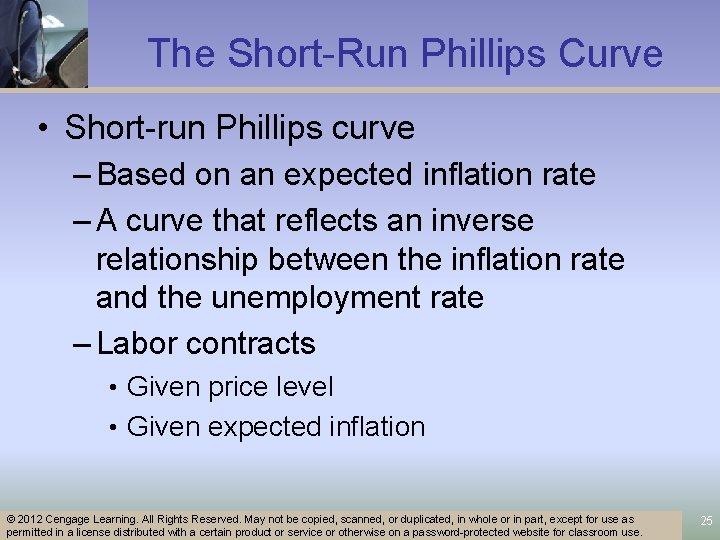
The Short-Run Phillips Curve • Short-run Phillips curve – Based on an expected inflation rate – A curve that reflects an inverse relationship between the inflation rate and the unemployment rate – Labor contracts • Given price level • Given expected inflation © 2012 Cengage Learning. All Rights Reserved. May not be copied, scanned, or duplicated, in whole or in part, except for use as permitted in a license distributed with a certain product or service or otherwise on a password-protected website for classroom use. 25

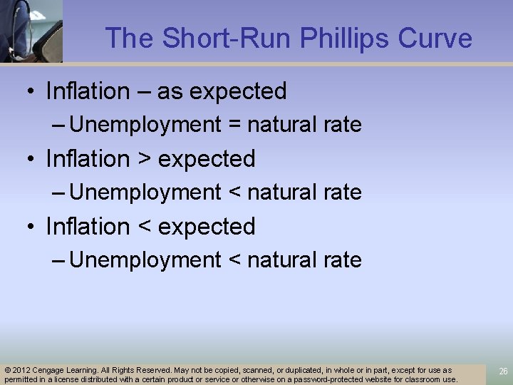
The Short-Run Phillips Curve • Inflation – as expected – Unemployment = natural rate • Inflation > expected – Unemployment < natural rate • Inflation < expected – Unemployment < natural rate © 2012 Cengage Learning. All Rights Reserved. May not be copied, scanned, or duplicated, in whole or in part, except for use as permitted in a license distributed with a certain product or service or otherwise on a password-protected website for classroom use. 26

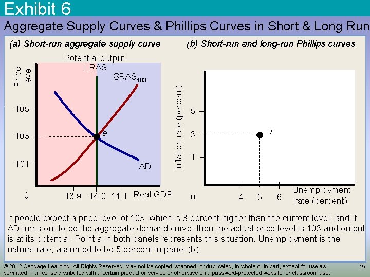
Exhibit 6 Aggregate Supply Curves & Phillips Curves in Short & Long Run Potential output LRAS SRAS 103 105 103 101 0 (b) Short-run and long-run Phillips curves a AD 13. 9 14. 0 14. 1 Real GDP Inflation rate (percent) Price level (a) Short-run aggregate supply curve 5 a 3 1 0 4 5 6 Unemployment rate (percent) If people expect a price level of 103, which is 3 percent higher than the current level, and if AD turns out to be the aggregate demand curve, then the actual price level is 103 and output is at its potential. Point a in both panels represents this situation. Unemployment is the natural rate, assumed to be 5 percent in panel (b). © 2012 Cengage Learning. All Rights Reserved. May not be copied, scanned, or duplicated, in whole or in part, except for use as permitted in a license distributed with a certain product or service or otherwise on a password-protected website for classroom use. 27

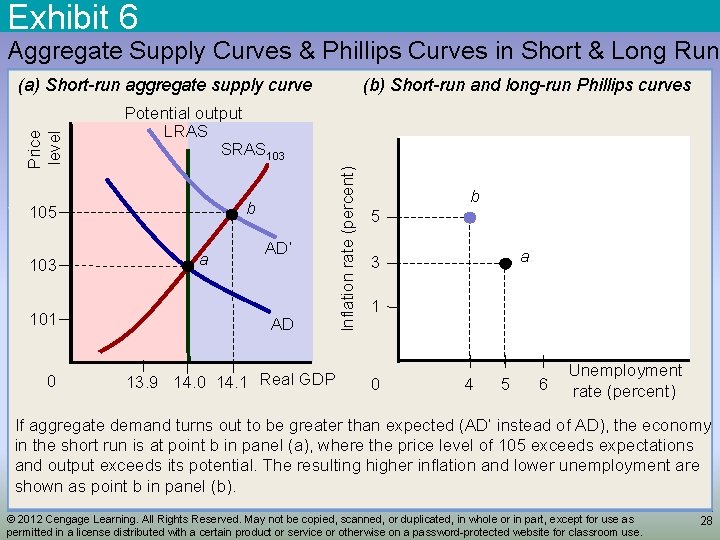
Exhibit 6 Aggregate Supply Curves & Phillips Curves in Short & Long Run Potential output LRAS SRAS 103 b 105 103 101 0 (b) Short-run and long-run Phillips curves a AD’ AD 13. 9 14. 0 14. 1 Real GDP Inflation rate (percent) Price level (a) Short-run aggregate supply curve b 5 a 3 1 0 4 5 6 Unemployment rate (percent) If aggregate demand turns out to be greater than expected (AD’ instead of AD), the economy in the short run is at point b in panel (a), where the price level of 105 exceeds expectations and output exceeds its potential. The resulting higher inflation and lower unemployment are shown as point b in panel (b). © 2012 Cengage Learning. All Rights Reserved. May not be copied, scanned, or duplicated, in whole or in part, except for use as permitted in a license distributed with a certain product or service or otherwise on a password-protected website for classroom use. 28

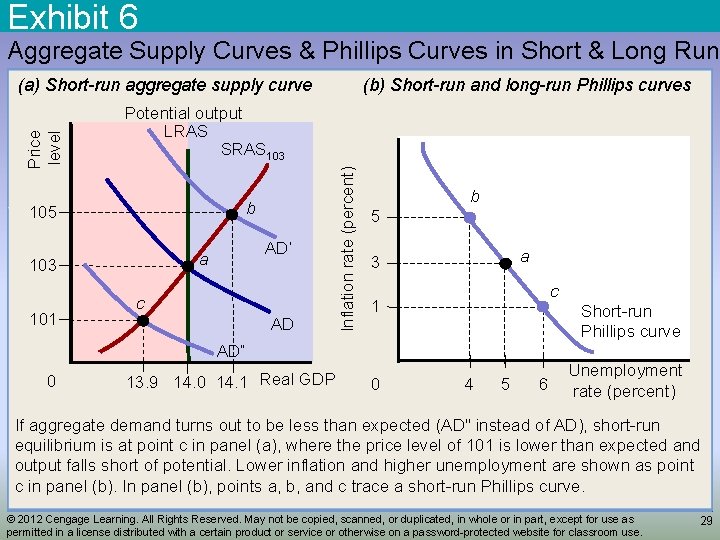
Exhibit 6 Aggregate Supply Curves & Phillips Curves in Short & Long Run Potential output LRAS SRAS 103 b 105 AD’ a 103 101 (b) Short-run and long-run Phillips curves c AD Inflation rate (percent) Price level (a) Short-run aggregate supply curve b 5 a 3 c 1 Short-run Phillips curve AD” 0 13. 9 14. 0 14. 1 Real GDP 0 4 5 6 Unemployment rate (percent) If aggregate demand turns out to be less than expected (AD" instead of AD), short-run equilibrium is at point c in panel (a), where the price level of 101 is lower than expected and output falls short of potential. Lower inflation and higher unemployment are shown as point c in panel (b). In panel (b), points a, b, and c trace a short-run Phillips curve. © 2012 Cengage Learning. All Rights Reserved. May not be copied, scanned, or duplicated, in whole or in part, except for use as permitted in a license distributed with a certain product or service or otherwise on a password-protected website for classroom use. 29

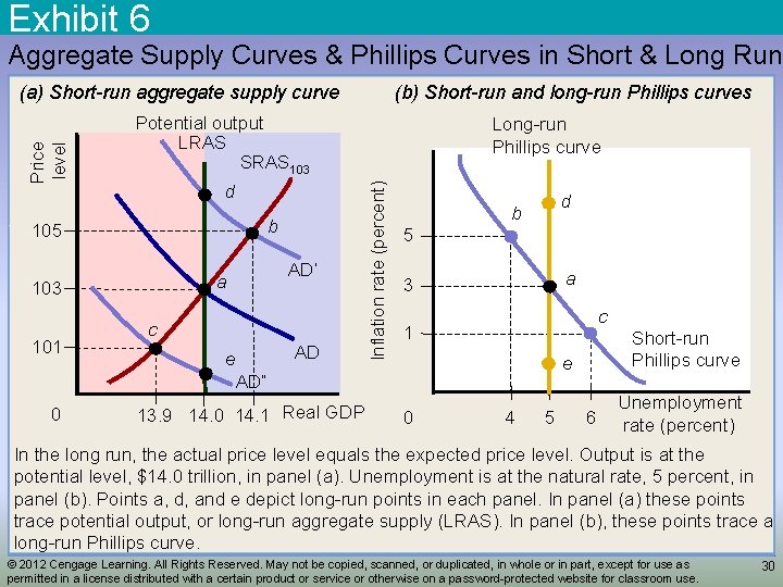
Exhibit 6 Aggregate Supply Curves & Phillips Curves in Short & Long Run Potential output LRAS SRAS 103 d b 105 AD’ a 103 101 (b) Short-run and long-run Phillips curves c AD e Long-run Phillips curve Inflation rate (percent) Price level (a) Short-run aggregate supply curve d b 5 a 3 c 1 e AD” 0 13. 9 14. 0 14. 1 Real GDP Short-run Phillips curve 0 4 5 6 Unemployment rate (percent) In the long run, the actual price level equals the expected price level. Output is at the potential level, $14. 0 trillion, in panel (a). Unemployment is at the natural rate, 5 percent, in panel (b). Points a, d, and e depict long-run points in each panel. In panel (a) these points trace potential output, or long-run aggregate supply (LRAS). In panel (b), these points trace a long-run Phillips curve. © 2012 Cengage Learning. All Rights Reserved. May not be copied, scanned, or duplicated, in whole or in part, except for use as permitted in a license distributed with a certain product or service or otherwise on a password-protected website for classroom use. 30

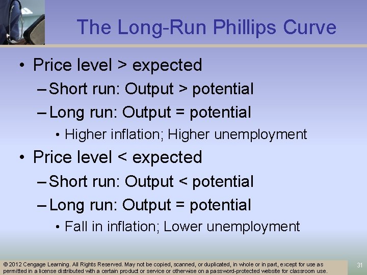
The Long-Run Phillips Curve • Price level > expected – Short run: Output > potential – Long run: Output = potential • Higher inflation; Higher unemployment • Price level < expected – Short run: Output < potential – Long run: Output = potential • Fall in inflation; Lower unemployment © 2012 Cengage Learning. All Rights Reserved. May not be copied, scanned, or duplicated, in whole or in part, except for use as permitted in a license distributed with a certain product or service or otherwise on a password-protected website for classroom use. 31

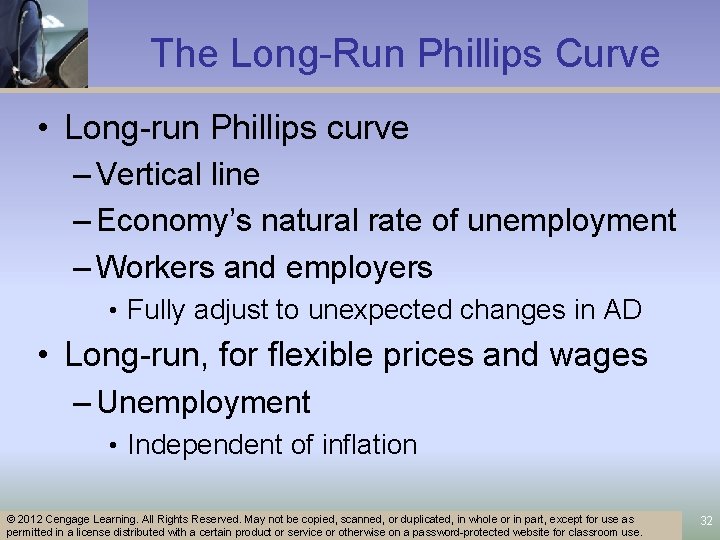
The Long-Run Phillips Curve • Long-run Phillips curve – Vertical line – Economy’s natural rate of unemployment – Workers and employers • Fully adjust to unexpected changes in AD • Long-run, for flexible prices and wages – Unemployment • Independent of inflation © 2012 Cengage Learning. All Rights Reserved. May not be copied, scanned, or duplicated, in whole or in part, except for use as permitted in a license distributed with a certain product or service or otherwise on a password-protected website for classroom use. 32

The Natural Rate Hypothesis • Long-run – Natural rate of unemployment – Independent of AD stimulus • Fiscal policy • Monetary policy • Optimal policy in long-run – Results in low inflation © 2012 Cengage Learning. All Rights Reserved. May not be copied, scanned, or duplicated, in whole or in part, except for use as permitted in a license distributed with a certain product or service or otherwise on a password-protected website for classroom use. 33

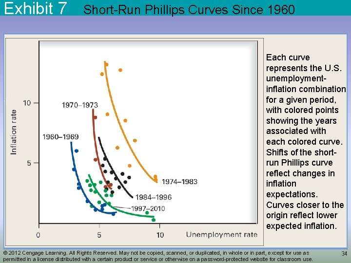
Exhibit 7 Short-Run Phillips Curves Since 1960 Each curve represents the U. S. unemploymentinflation combination for a given period, with colored points showing the years associated with each colored curve. Shifts of the shortrun Phillips curve reflect changes in inflation expectations. Curves closer to the origin reflect lower expected inflation. © 2012 Cengage Learning. All Rights Reserved. May not be copied, scanned, or duplicated, in whole or in part, except for use as permitted in a license distributed with a certain product or service or otherwise on a password-protected website for classroom use. 34