Path Analysis SASCalis Theory of Planned Behavior Note

Path Analysis SAS/Calis

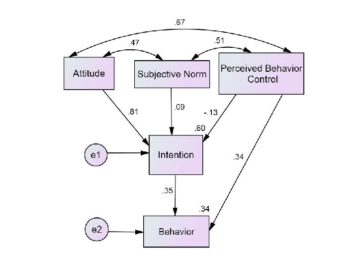
Theory of Planned Behavior Note that this model is not saturated.

Zero-Order Correlations Attitude Sub. Norm Attitude PBC Intent Behavior 1. 000 . 472 . 665 . 767 . 525 Sub. Norm . 472 1. 000 . 505 . 411 . 379 PBC . 665 . 505 1. 000 . 458 . 496 Intent . 767 . 411 . 458 1. 000 . 503 Behavior . 525 . 379 . 496 . 503 1. 000

Read in the Data options formdlim='-' nodate pagno=min; TITLE 'Path Analysis, Ingram Data' ; data Ingram(type=corr); INPUT _TYPE_ $ _NAME_ $ Attitude Sub. Norm PBC Intent Behavior; CARDS;

N. 60 60 60 MEAN. 32. 02 45. 71 40. 25 16. 92 43. 92 STD. 6. 96 12. 32 7. 62 3. 83 16. 66 CORR Attitude 1. 472. 665. 767. 525 CORR Subnorm. 472 1. 505. 411. 379 CORR PBC. 665. 505 1. 458. 496 CORR Intent. 767. 411. 458 1. 503 CORR Behavior. 525. 379. 496. 503 1

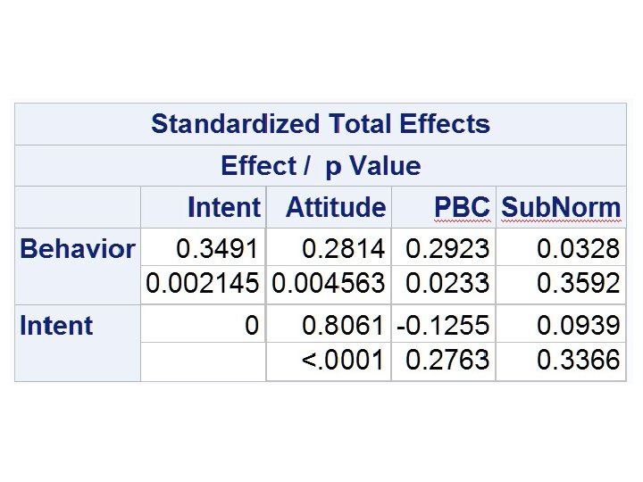
Conduct the Analysis Proc Calis PRINT; • PRINT adds to the default output the total effects matrix (and some other things)

Linear Equations LINEQS Intent = b 1 Attitude + b 2 Sub. Norm + b 3 PBC + E 1, • Intent has paths to it from Attitude, Sub. Norm, PBC, and E 1 (the error term) • b 1, b 2, and b 3 are the path coefficients that we want SAS to estimate for us

Linear Equations Behavior = b 4 Intent + b 5 PBC + E 2; • Behavior has paths to it from Intent, PBC, and E 2. • SAS assumes that the exogenous variables (Attitude, Sub. Norm, and PBC) are correlated.

Linear Equations STD E 1 -E 2 = V 1 -V 2; run; • The error terms be estimated as parameters V 1 and V 2.

The Output • The complete output is available online. • Here I shall present the key parts of the output.

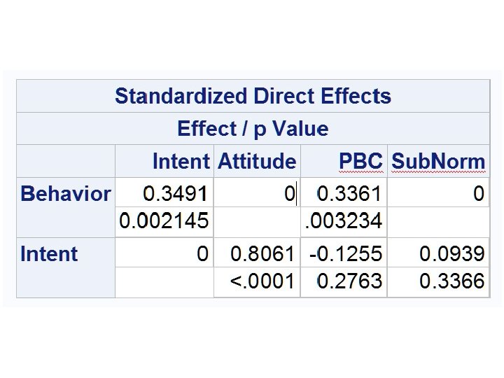
The Path Coefficients Standardized Results for Linear Equations Intent = 0. 8061 * Attitude + 0. 0939 Behavior = 0. 3491 * Intent + 0. 3361 * Sub. Norm + -0. 1255 * PBC

Standardized Error Coefficients Variable E 1 E 2 Parameter V 1 V 2 Estimate 0. 40058 0. 65770

Standardized Coefficients Among Exogenous Variables Var 1 Sub. Norm PBC Var 2 Attitude Sub. Norm Estimate 0. 47200 0. 66500 0. 50500

Fit Summary Chi-Square 0. 8564 Chi-Square DF 2 above. 05 is good Pr > Chi-Square 0. 6517 below. 08 is good Standardized RMSR (SRMSR) 0. 0191 above. 95 is good Goodness of Fit Index (GFI) 0. 9943 below. 01 is excellent RMSEA Estimate 0. 0000 above. 05 is good Probability of Close Fit 0. 6905 above. 95 is good Bentler Comparative Fit Index 1. 0000 above. 95 is good Bentler-Bonett NFI 0. 9936

Goodness of Fit Indices • http: //core. ecu. edu/psyc/wuenschk/MV/SE M/Goodness-Fit_SEM. docx
- Slides: 19