Optimal PowerDown Strategies Chaitanya Swamy Caltech John Augustine

Optimal Power-Down Strategies Chaitanya Swamy Caltech John Augustine Sandy Irani University of California, Irvine

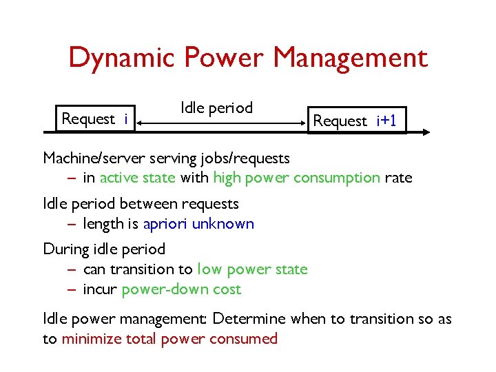
Dynamic Power Management Request i Idle period Request i+1 Machine/server serving jobs/requests – in active state with high power consumption rate Idle period between requests – length is apriori unknown During idle period – can transition to low power state – incur power-down cost Idle power management: Determine when to transition so as to minimize total power consumed

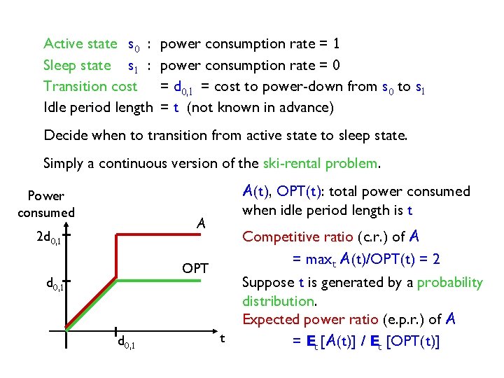
Active state s 0 : Sleep state s 1 : Transition cost Idle period length power consumption rate = 1 power consumption rate = 0 = d 0, 1 = cost to power-down from s 0 to s 1 = t (not known in advance) Decide when to transition from active state to sleep state. Simply a continuous version of the ski-rental problem. Power consumed A(t), OPT(t): total power consumed when idle period length is t A 2 d 0, 1 Competitive ratio (c. r. ) of A = maxt A(t)/OPT(t) = 2 OPT d 0, 1 t Suppose t is generated by a probability distribution. Expected power ratio (e. p. r. ) of A = Et [A(t)] / Et [OPT(t)]

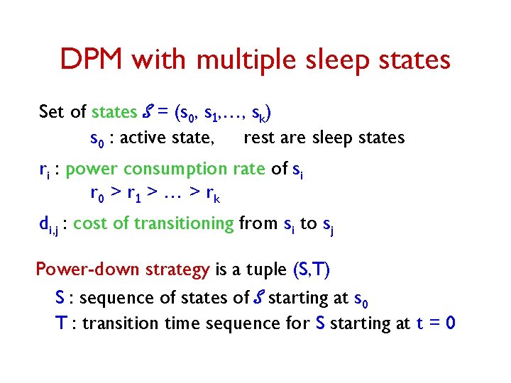
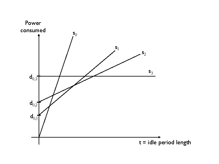
DPM with multiple sleep states Set of states S = (s 0, s 1, …, sk) s 0 : active state, rest are sleep states ri : power consumption rate of si r 0 > r 1 > … > rk di, j : cost of transitioning from si to sj Power-down strategy is a tuple (S, T) S : sequence of states of S starting at s 0 T : transition time sequence for S starting at t = 0

Power consumed s 0 s 1 d 0, 3 s 2 s 3 d 0, 2 d 0, 1 t = idle period length

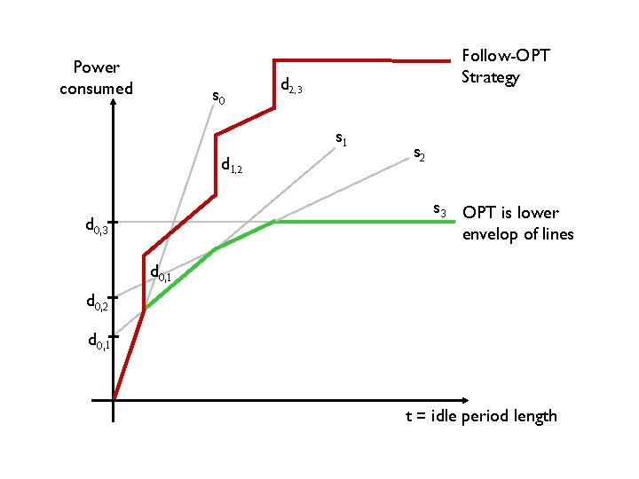
Power consumed s 0 Follow-OPT Strategy d 2, 3 s 1 d 1, 2 s 3 OPT is lower envelop of lines d 0, 3 d 0, 1 d 0, 2 d 0, 1 t = idle period length

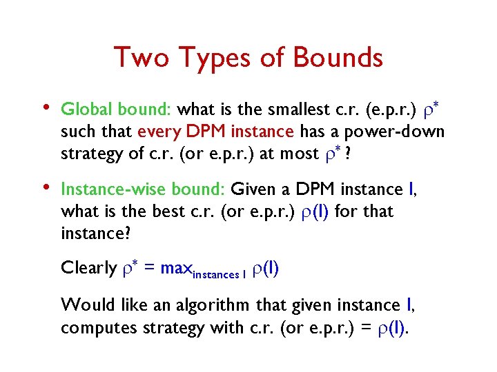
Two Types of Bounds • Global bound: what is the smallest c. r. (e. p. r. ) r* such that every DPM instance has a power-down strategy of c. r. (or e. p. r. ) at most r* ? • Instance-wise bound: Given a DPM instance I, what is the best c. r. (or e. p. r. ) r(I) for that instance? Clearly r* = maxinstances I r(I) Would like an algorithm that given instance I, computes strategy with c. r. (or e. p. r. ) = r(I).

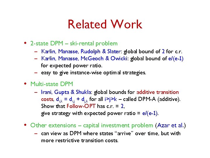
Related Work • 2 -state DPM – ski-rental problem – Karlin, Manasse, Rudolph & Slater: global bound of 2 for c. r. – Karlin, Manasse, Mc. Geoch & Owicki: global bound of e/(e-1) for expected power ratio. – easy to give instance-wise optimal strategies. • Multi-state DPM – Irani, Gupta & Shukla: global bounds for additive transition costs, di, k = di, j + dj, k for all i>j>k – called DPM-A (additive). Show that Follow-OPT has c. r. = 2, give strategy with expected power ratio = e/(e-1). • Other extensions – capital investment problem (Azar et al. ) – can view as DPM where states “arrive” over time, but with more restrictive transition costs.

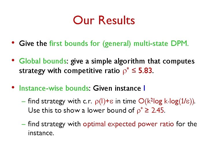
Our Results • Give the first bounds for (general) multi-state DPM. • Global bounds: give a simple algorithm that computes strategy with competitive ratio r* ≤ 5. 83. • Instance-wise bounds: Given instance I – find strategy with c. r. r(I)+e in time O(k 2 log k. log(1/e)). Use this to show a lower bound of r* ≥ 2. 45. – find strategy with optimal expected power ratio for the instance.

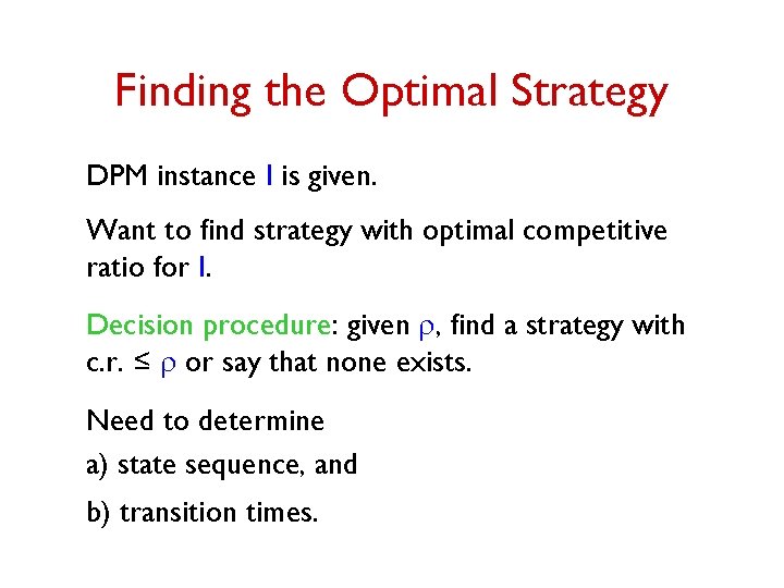
Finding the Optimal Strategy DPM instance I is given. Want to find strategy with optimal competitive ratio for I. Decision procedure: given r, find a strategy with c. r. ≤ r or say that none exists. Need to determine a) state sequence, and b) transition times.

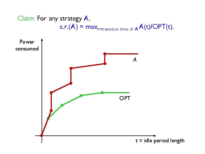
Claim: For any strategy A, c. r. (A) = maxt=transition time of A A(t)/OPT(t). Power consumed A OPT t = idle period length

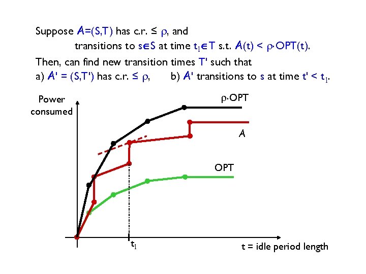
Suppose A=(S, T) has c. r. ≤ r, and transitions to sÎS at time t 1ÎT s. t. A(t) < r. OPT(t). Then, can find new transition times T' such that a) A' = (S, T') has c. r. ≤ r, b) A' transitions to s at time t' < t 1. r. OPT Power consumed A OPT t 1 t = idle period length

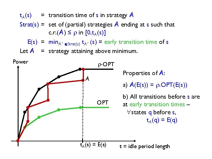
t. A(s) = transition time of s in strategy A Strat(s) = set of (partial) strategies A ending at s such that c. r. (A) ≤ r in [0, t. A(s)] E(s) = min. A' ÎStrat(s) t. A' (s) = early transition time of s Let A = strategy attaining above minimum. Power r. OPT Properties of A: A a) A(E(s)) = r. OPT(E(s)) OPT t. A(s) = E(s) b) All transitions before s are at early transition times – "states q before s, t. A(q) = E(q) t = idle period length

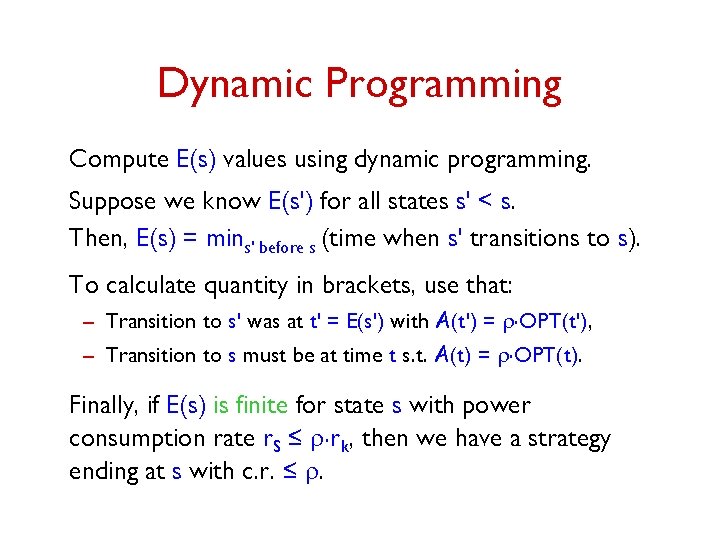
Dynamic Programming Compute E(s) values using dynamic programming. Suppose we know E(s') for all states s' < s. Then, E(s) = mins' before s (time when s' transitions to s). To calculate quantity in brackets, use that: – Transition to s' was at t' = E(s') with A(t') = r. OPT(t'), – Transition to s must be at time t s. t. A(t) = r. OPT(t). Finally, if E(s) is finite for state s with power consumption rate r. S ≤ r. rk, then we have a strategy ending at s with c. r. ≤ r.

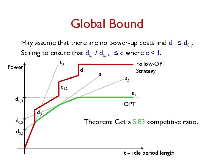
Global Bound May assume that there are no power-up costs and di, j ≤ d 0, j. Scaling to ensure that d 0, i / d 0, i+1 ≤ c where c < 1. s 0 Power d 1, 2 d 0, 3 d 2, 3 s 1 Follow-OPT Strategy s 2 s 3 OPT d 0, 1 d 0, 2 Theorem: Get a 5. 83 competitive ratio. d 0, 1 t = idle period length

Open Questions • Randomized strategies: global or instance-wise bounds for randomized strategies. • Better lower bounds.

Thank You.