Network Design for Information Networks Chaitanya Swamy Caltech

Network Design for Information Networks Chaitanya Swamy Caltech and U. Waterloo Ara Hayrapetyan Éva Tardos Cornell University

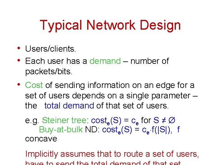
Typical Network Design • Users/clients. • Each user has a demand – number of packets/bits. • Cost of sending information on an edge for a set of users depends on a single parameter – the total demand of that set of users. e. g. Steiner tree: coste(S) = ce for S ≠ Ø Buy-at-bulk ND: coste(S) = ce. f(|S|), f concave Implicitly assumes that to route a set of users,

Information Aggregation Model • Take a higher level view – want to capture • • information aggregation. Each user has some information. Interested in the total information flow of a set of users allowing for information aggregation. q cost of sending information of a set of users could be much less than the sum of the individual information needs incur cost savings q some information may aggregate better than others aggregation/cost function depends on the set of users • Can capture complex relations between users by using a set-based cost function.

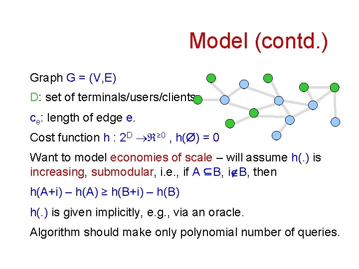
Model (contd. ) Graph G = (V, E) D: set of terminals/users/clients. ce: length of edge e. Cost function h : 2 D ® ≥ 0 , h(Ø) = 0 Want to model economies of scale – will assume h(. ) is increasing, submodular, i. e. , if A Í B, iÏB, then h(A+i) – h(A) ≥ h(B+i) – h(B) h(. ) is given implicitly, e. g. , via an oracle. Algorithm should make only polynomial number of queries.

Applicability • Sensor Networks – Distributed sensor nodes send information to central node(s) – Information can often be well aggregated along paths, e. g. , temperature readings – May care only about aggregate information, e. g. , average temperature, humidity … • Content-based publish-subscribe systems – Users “publish” or “subscribe” to information – Information flowing through network can be aggregated

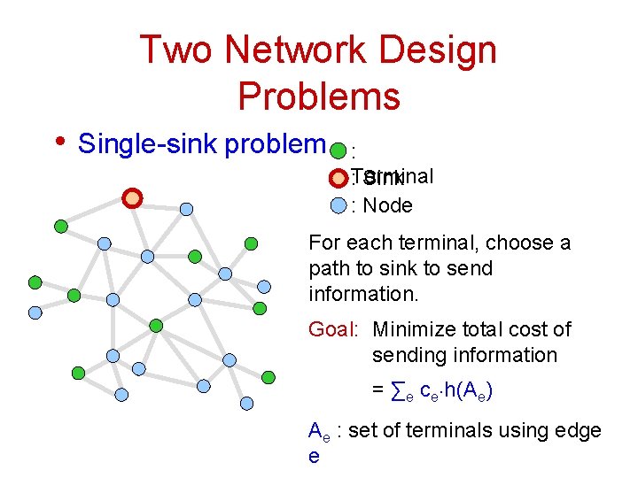
Two Network Design Problems • Single-sink problem : : Terminal Sink : Node For each terminal, choose a path to sink to send information. Goal: Minimize total cost of sending information = ∑e ce. h(Ae) Ae : set of terminals using edge e

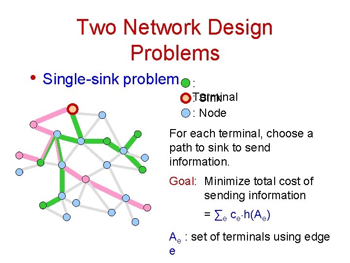
Two Network Design Problems • Single-sink problem : : Terminal Sink : Node For each terminal, choose a path to sink to send information. Goal: Minimize total cost of sending information = ∑e ce. h(Ae) Ae : set of terminals using edge e

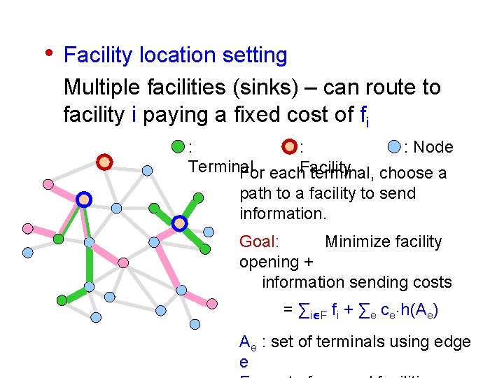
• Facility location setting Multiple facilities (sinks) – can route to facility i paying a fixed cost of fi : : : Node Terminal For each. Facility terminal, choose a path to a facility to send information. Goal: Minimize facility opening + information sending costs = ∑iÎF fi + ∑e ce. h(Ae) Ae : set of terminals using edge e

General problem includes many interesting problem classes. • Buy-at-bulk network design. • Facility location with buy-at-bulk connection costs – includes uncapacitated facility location. • Dependent Maybecast – generalization of Karger-Minkoff (KM 00) maybecast problem. • 2 -stage stochastic Steiner tree problem. • Well-approximates the multi-stage Stochastic Steiner tree problem. • Interval routing problem (Williamson et al. ): each user has to send an interval to the root on a single path; cost of e = total length of intervals sent on it

Our Results • Give an O(log |V|)-approximation for the general problem using tree embeddings. • Obtain a 4 -approximation for Group Facility Location: – terminals divided into groups; cost of e = ce. (# of groups using e) have to open facilities and connect each group to open facilities via a Steiner forest. Algorithm combines [AKR, GW]-algorithm for Steiner forest and JV-algorithm for facility location via a novel cleanup phase. • Give an O(k)-approximation for Dependent Maybecast (probabilistic Steiner tree) with k-level distribution tree. • Get a 2 k-approximation for k-stage Steiner tree

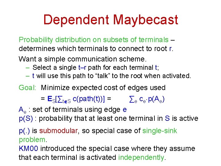
Dependent Maybecast Probability distribution on subsets of terminals – determines which terminals to connect to root r. Want a simple communication scheme. – Select a single t–r path for each terminal t; – t will use this path to “talk” to the root when activated. Goal: Minimize expected cost of edges used = ES[∑tÎS c(path(t))] = ∑e ce. p(Ae) Ae : set of terminals using edge e p(S) : probability that at least one terminal in S is active p(. ) is submodular, so special case of single-sink problem. KM 00 introduced the special case where they assume that each terminal is activated independently.

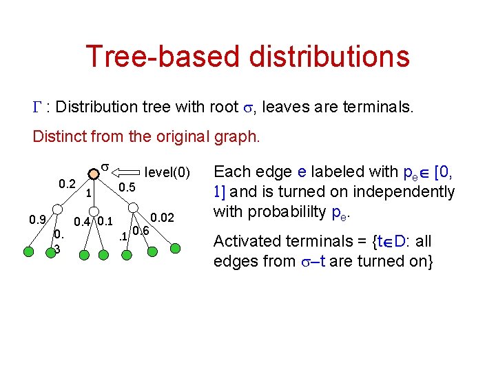
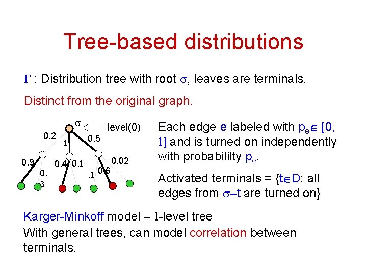
Tree-based distributions G : Distribution tree with root s, leaves are terminals. Distinct from the original graph. s 0. 2 0. 9 0. 3 1 0. 4 0. 1 level(0) 0. 5. 1 0. 6 0. 02 Each edge e labeled with peÎ [0, 1] and is turned on independently with probabililty pe. Activated terminals = {tÎD: all edges from s–t are turned on}

Tree-based distributions G : Distribution tree with root s, leaves are terminals. Distinct from the original graph. s 0. 2 0. 9 0. 3 1 0. 4 0. 1 level(0) 0. 5. 1 0. 6 0. 02 Each edge e labeled with peÎ [0, 1] and is turned on independently with probabililty pe. Activated terminals = {tÎD: all edges from s–t are turned on} Karger-Minkoff model º 1 -level tree With general trees, can model correlation between terminals.

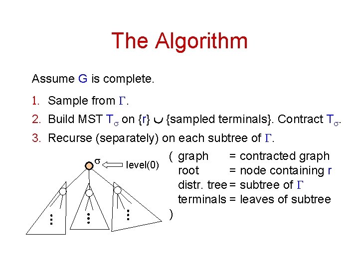
The Algorithm Assume G is complete. 1. Sample from G. 2. Build MST Ts on {r} È {sampled terminals}. Contract Ts. 3. Recurse (separately) on each subtree of G. s ( graph = contracted graph level(0) root = node containing r distr. tree = subtree of G terminals = leaves of subtree )

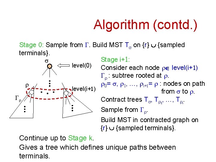
Algorithm (contd. ) Stage 0: Sample from G. Build MST Ts on {r} È {sampled terminals}. Stage i+1: s level(0) Consider each node rÎ level(i+1) Gr : subtree rooted at r. r 0= s, r 1, …, ri+1= r : nodes on path r level(i+1) from s to r. Gr Contract trees Ts, Tr 1, …, Tri. Sample from Gr. Build MST in contracted graph on {r} È {sampled terminals}. Continue up to Stage k. Gives a tree which defines unique paths between terminals.

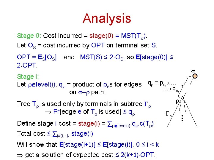
Analysis Stage 0: Cost incurred = stage(0) = MST(Ts). Let OS = cost incurred by OPT on terminal set S. OPT = ES[OS] 2. OPT. and MST(S) ≤ 2. OS, so E[stage(0)] ≤ Stage i: Let rÎlevel(i), qr = product of pes for edges qr = pe x … … x pe on s–r path. s 1 Tree Tr is used only by terminals in subtree Gr Pr[edge e of Tr is used] ≤ qr Define stage i cost = stage(i) = ∑rÎlevel(i) qr. c(Tr) Total cost ≤ ∑i=0…k stage(i) Will show that E[stage(i+1)] ≤ E[stage(i)], 0 ≤ i < k get a solution of expected cost ≤ 2(k+1). OPT. i r Gr

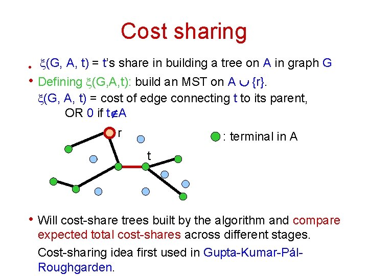
Cost sharing • x(G, A, t) = t’s share in building a tree on A in graph G • Defining x(G, A, t): build an MST on A È {r}. x(G, A, t) = cost of edge connecting t to its parent, OR 0 if tÏA r : terminal in A t • Will cost-share trees built by the algorithm and compare expected total cost-shares across different stages. Cost-sharing idea first used in Gupta-Kumar-Pál. Roughgarden.

E[stage(i+1)] ≤ E[stage(i)] Show this for i=0. Consider node r Î level(1). Condition on set H' = nodes from G' picked in stage 0. Let S = nodes “attached” to r in stage 0. Same random process determines S in stage 0 and stage 1. s Cost share (CS) of S in stage 0 e r G' = 0 if e is not “on”, ∑tÎS x(G, H' È S, t) otherwise. Gr H' S CS of S in stage 1 = ∑tÎS x(G/H, S, t) where H H' =≤ terminals ∑tÎS x(G/H, S, t) = cost(MST(S) in Ê G/H) ∑tÎS x(G, H' È S, activated in stage 0 t)

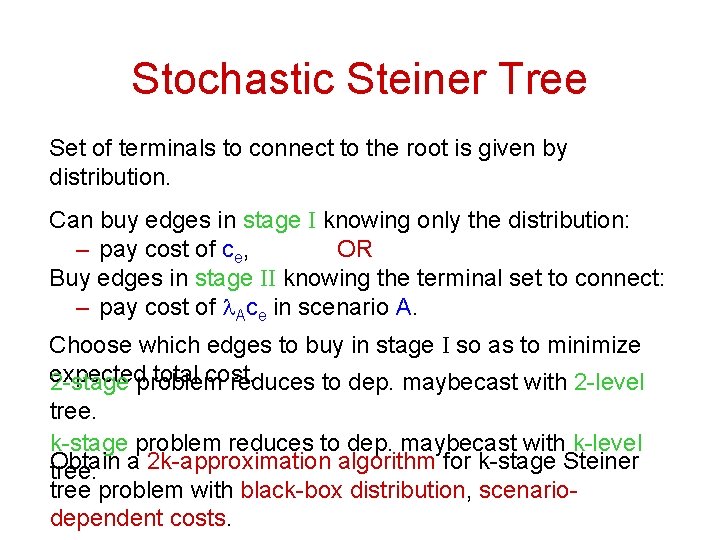
Stochastic Steiner Tree Set of terminals to connect to the root is given by distribution. Can buy edges in stage I knowing only the distribution: – pay cost of ce, OR Buy edges in stage II knowing the terminal set to connect: – pay cost of l. Ace in scenario A. Choose which edges to buy in stage I so as to minimize expected total cost. 2 -stage problem reduces to dep. maybecast with 2 -level tree. k-stage problem reduces to dep. maybecast with k-level Obtain tree. a 2 k-approximation algorithm for k-stage Steiner tree problem with black-box distribution, scenariodependent costs.

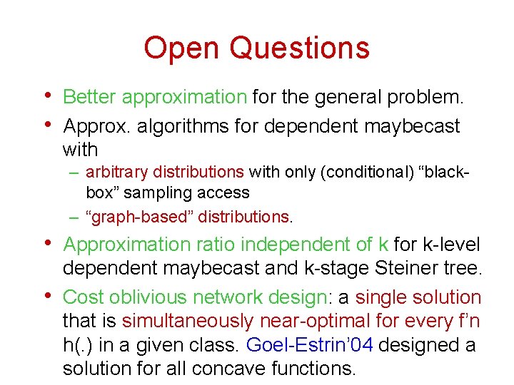
Open Questions • Better approximation for the general problem. • Approx. algorithms for dependent maybecast with – arbitrary distributions with only (conditional) “blackbox” sampling access – “graph-based” distributions. • Approximation ratio independent of k for k-level • dependent maybecast and k-stage Steiner tree. Cost oblivious network design: a single solution that is simultaneously near-optimal for every f’n h(. ) in a given class. Goel-Estrin’ 04 designed a solution for all concave functions.

Thank You.