Operations Management Performance Modeling 1 Operations Strategy 2

Operations Management & Performance Modeling 1 Operations Strategy 2 Process Analysis 3 Lean Operations 4 Supply Chain Management – Class 5 a: Inventories & Economies of Scale – Class 5 b: Dealing with Uncertainty & role of Centralization » The impact of uncertainty: safety stocks » Centralization: pooling benefits 5 Capacity Management in Services 6 Total Quality Management 7 Business Process Reengineering OM&PM/Class 5 b 1

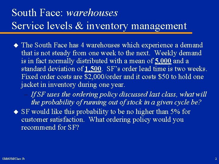
South Face: warehouses Service levels & inventory management u u The South Face has 4 warehouses which experience a demand that is not steady from one week to the next. Weekly demand is in fact normally distributed with a mean of 5, 000 and a standard deviation of 1, 500. SF’s order lead time is two weeks. Fixed order costs are $2, 000/order and it costs $50 to hold one jacket in inventory during one year. – If SF uses the ordering policy discussed last class, what will the probability of running out of stock in a given cycle be? SF would like this probability to be no higher than 5% for customer satisfaction. What ordering policy would you recommend for SF? OM&PM/Class 5 b 2

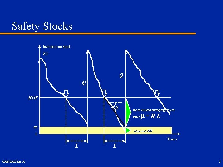
Safety Stocks Inventory on hand I(t) Q Q order ROP R mean demand during supply lead time: ss m=RL safety stock 0 ss Time t L OM&PM/Class 5 b L 3

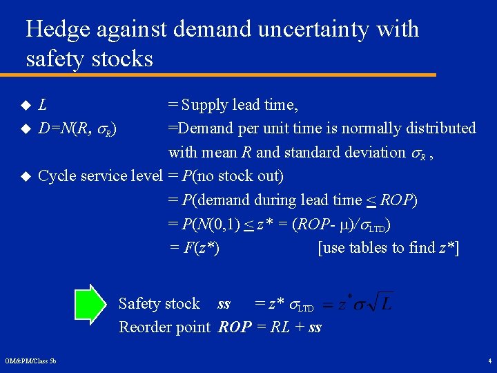
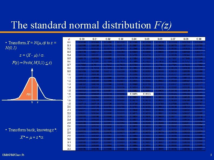
Hedge against demand uncertainty with safety stocks u u u L D=N(R, s. R) = Supply lead time, =Demand per unit time is normally distributed with mean R and standard deviation s. R , Cycle service level = P(no stock out) = P(demand during lead time < ROP) = P(N(0, 1) < z* = (ROP- m)/s. LTD) = F(z*) [use tables to find z*] Safety stock ss = z* s. LTD Reorder point ROP = RL + ss OM&PM/Class 5 b 4

The standard normal distribution F(z) • Transform X = N(m, s) to z = N(0, 1) z = (X - m) / s. F(z) = Prob( N(0, 1) < z) F(z) 0 z • Transform back, knowing z*: X* = m + z*s. OM&PM/Class 5 b 5

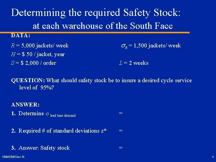
Determining the required Safety Stock: at each warehouse of the South Face DATA: R = 5, 000 jackets/ week H = $ 50 / jacket, year S = $ 2, 000 / order s. R = 1, 500 jackets/ week L = 2 weeks QUESTION: What should safety stock be to insure a desired cycle service level of 95%? ANSWER: 1. Determine s lead time demand = 2. Required # of standard deviations z* = 3. Answer: Safety stock = OM&PM/Class 5 b 6

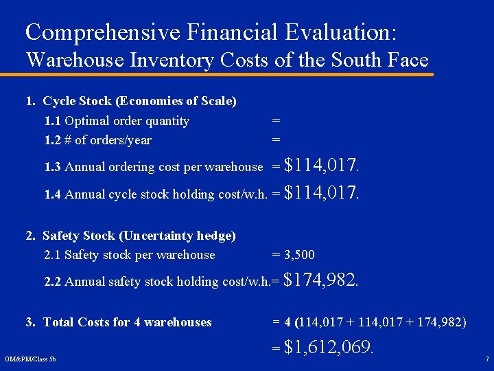
Comprehensive Financial Evaluation: Warehouse Inventory Costs of the South Face 1. Cycle Stock (Economies of Scale) 1. 1 Optimal order quantity 1. 2 # of orders/year = = 1. 3 Annual ordering cost per warehouse = $114, 017. 1. 4 Annual cycle stock holding cost/w. h. = $114, 017. 2. Safety Stock (Uncertainty hedge) 2. 1 Safety stock per warehouse = 3, 500 2. 2 Annual safety stock holding cost/w. h. = $174, 982. 3. Total Costs for 4 warehouses OM&PM/Class 5 b = 4 (114, 017 + 174, 982) = $1, 612, 069. 7

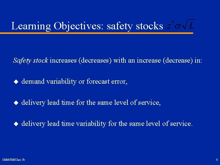
Learning Objectives: safety stocks Safety stock increases (decreases) with an increase (decrease) in: u demand variability or forecast error, u delivery lead time for the same level of service, u delivery lead time variability for the same level of service. OM&PM/Class 5 b 8

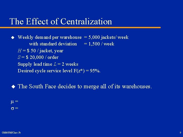
The Effect of Centralization u Weekly demand per warehouse = 5, 000 jackets/ week with standard deviation = 1, 500 / week H = $ 50 / jacket, year S = $ 20, 000 / order Supply lead time L = 2 weeks Desired cycle service level F(z*) = 95%. u The South Face decides to merge all of its warehouses. m= s= OM&PM/Class 5 b 9

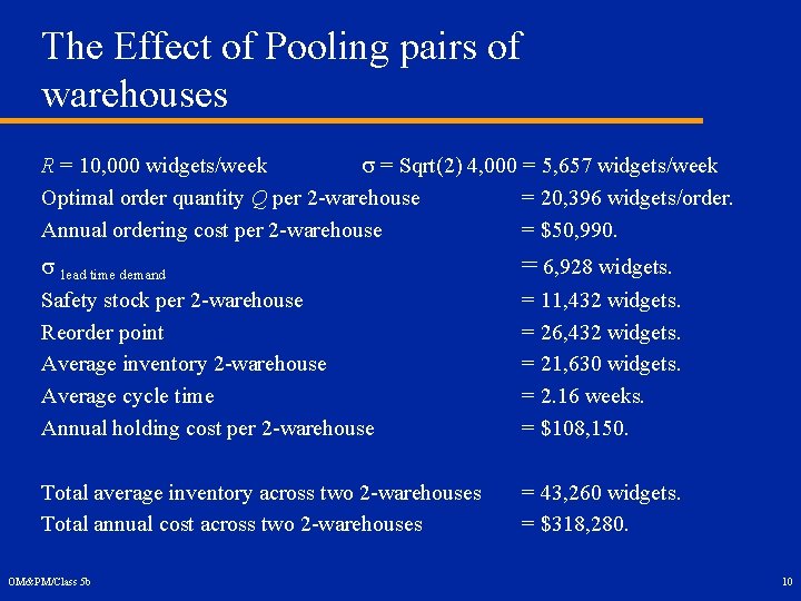
The Effect of Pooling pairs of warehouses R = 10, 000 widgets/week s = Sqrt(2) 4, 000 = 5, 657 widgets/week Optimal order quantity Q per 2 -warehouse = 20, 396 widgets/order. Annual ordering cost per 2 -warehouse = $50, 990. s lead time demand Safety stock per 2 -warehouse Reorder point Average inventory 2 -warehouse Average cycle time Annual holding cost per 2 -warehouse = 6, 928 widgets. Total average inventory across two 2 -warehouses Total annual cost across two 2 -warehouses = 43, 260 widgets. = $318, 280. OM&PM/Class 5 b = 11, 432 widgets. = 26, 432 widgets. = 21, 630 widgets. = 2. 16 weeks. = $108, 150. 10

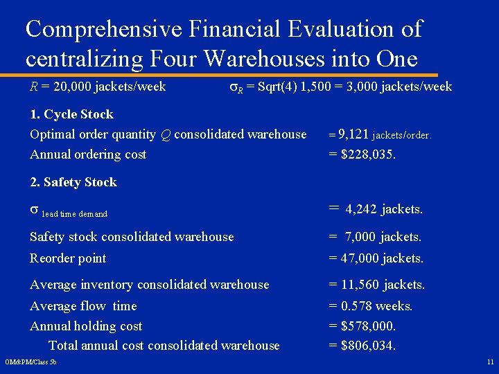
Comprehensive Financial Evaluation of centralizing Four Warehouses into One R = 20, 000 jackets/week s. R = Sqrt(4) 1, 500 = 3, 000 jackets/week 1. Cycle Stock Optimal order quantity Q consolidated warehouse Annual ordering cost = 9, 121 jackets/order. = $228, 035. 2. Safety Stock s lead time demand = 4, 242 jackets. Safety stock consolidated warehouse = 7, 000 jackets. Reorder point = 47, 000 jackets. Average inventory consolidated warehouse = 11, 560 jackets. Average flow time Annual holding cost Total annual cost consolidated warehouse = 0. 578 weeks. = $578, 000. = $806, 034. OM&PM/Class 5 b 11

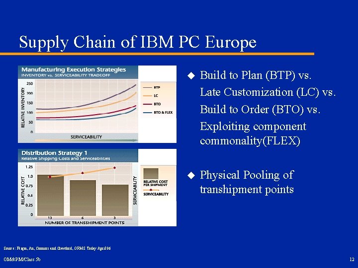
Supply Chain of IBM PC Europe u Build to Plan (BTP) vs. Late Customization (LC) vs. Build to Order (BTO) vs. Exploiting component commonality(FLEX) u Physical Pooling of transhipment points Source: Feigin, An, Connors and Crawford, ORMS Today April 96 OM&PM/Class 5 b 12

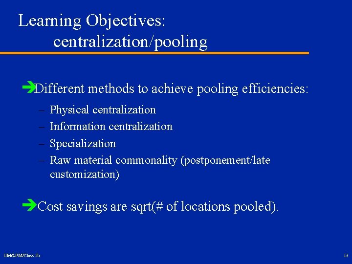
Learning Objectives: centralization/pooling èDifferent methods to achieve pooling efficiencies: – – Physical centralization Information centralization Specialization Raw material commonality (postponement/late customization) èCost savings are sqrt(# of locations pooled). OM&PM/Class 5 b 13