Neuse Estuary Eutrophication Model Predictions of Water Quality

Neuse Estuary Eutrophication Model: Predictions of Water Quality Improvement By James D. Bowen UNC Charlotte

Calibration Summary • Both transport and water quality model are able to simulate observed system dynamics • nutrients generally decreasing “downstream” • high nutrients may not immediately produce high chl-a

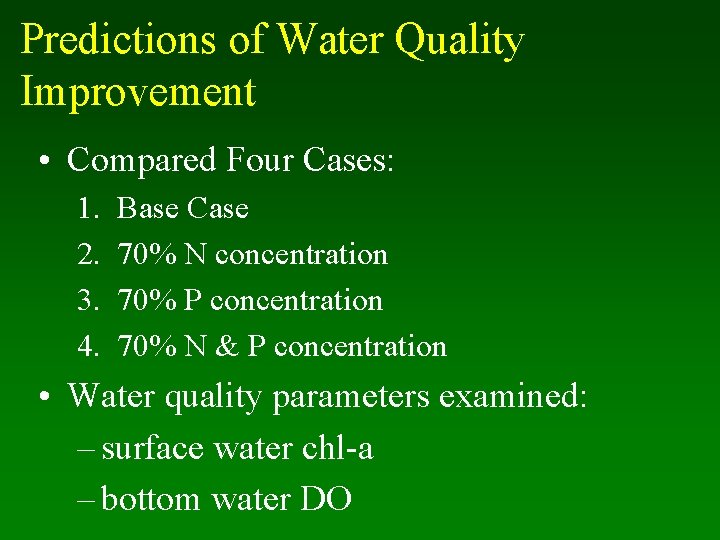
Predictions of Water Quality Improvement • Compared Four Cases: 1. 2. 3. 4. Base Case 70% N concentration 70% P concentration 70% N & P concentration • Water quality parameters examined: – surface water chl-a – bottom water DO

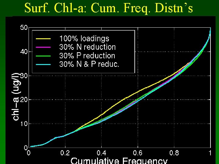
Surf. Chl-a: Cum. Freq. Distn’s

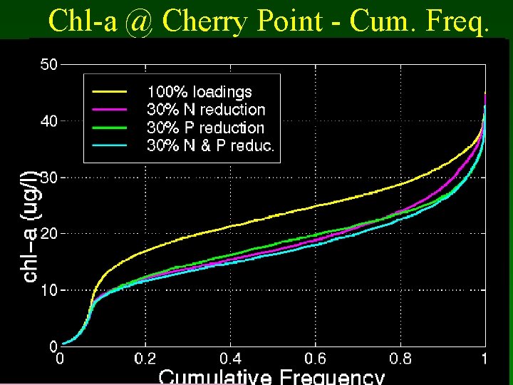
Chl-a @ Cherry Point - Cum. Freq.

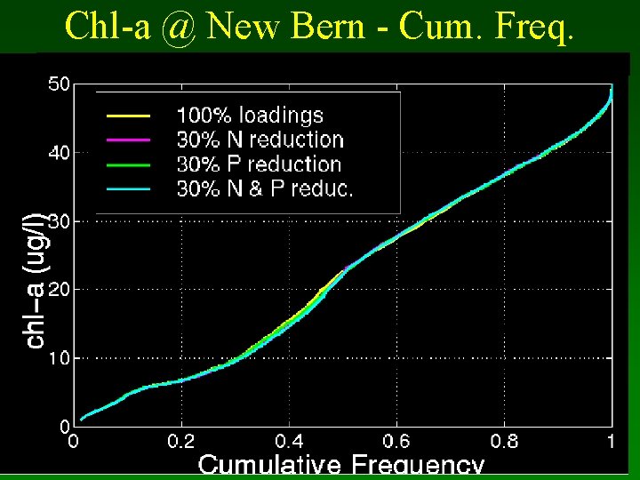
Chl-a @ New Bern - Cum. Freq.

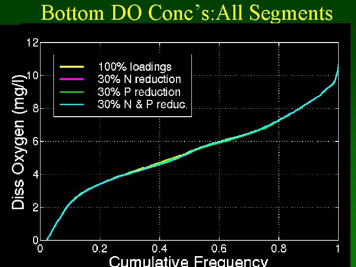
Bottom DO Conc’s: All Segments

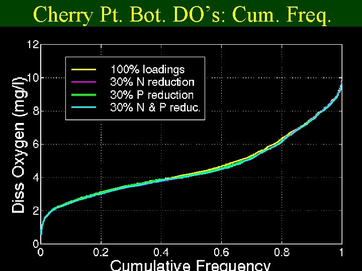
Cherry Pt. Bot. DO’s: Cum. Freq.

Bottom DO Conc’s: Lower Sed. Conc.

Another Special Feature of this Model Application Emphasis on quantifying modeling uncertainties

Uncertainty Analysis • Objective: put “error bars” on model predictions • Error sources: model error, boundary & initial conditions, parameter error • calibration performance gives estimate of model, boundary, and inital condition error • parameter error usually estimated with sensitivity analysis

Uncertainty Analysis • Standard sensitivity analysis: – vary model parameters one-by-one and measure variability in model predictions • Standard sensitivity analysis may under or over predict uncertainty • Basic problem: calibration and sensitivity analysis done as separate, independent procedures

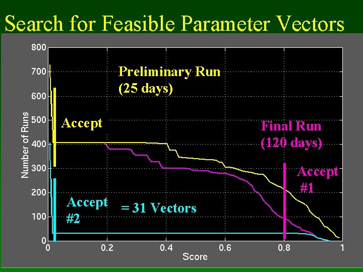
Uncertainty Analysis Method • Couple uncertainty analysis w/ calibration • Determine not one but many “feasible” parameter vectors • Each feasible vector produces desired system behavior – 31 of 729 were feasible • Run model w/ each feasible vector to determine specification uncertainty

Uncertainty Analysis • Prediction uncertainty = specification uncertainty + residual error • method similar to the “Regional Sensitivity Analysis” (Adams 1998) method used for Lake Okeechobee

Establishing System Behavior • Seasonal/Spatial Trends – based upon 1991 monitoring data – nutrients decreasing downstream – early mid-estuary phytoplankton bloom – later upper-estuary bloom – several pulses of high NOx conc. @ New Bern – DO decreases through season

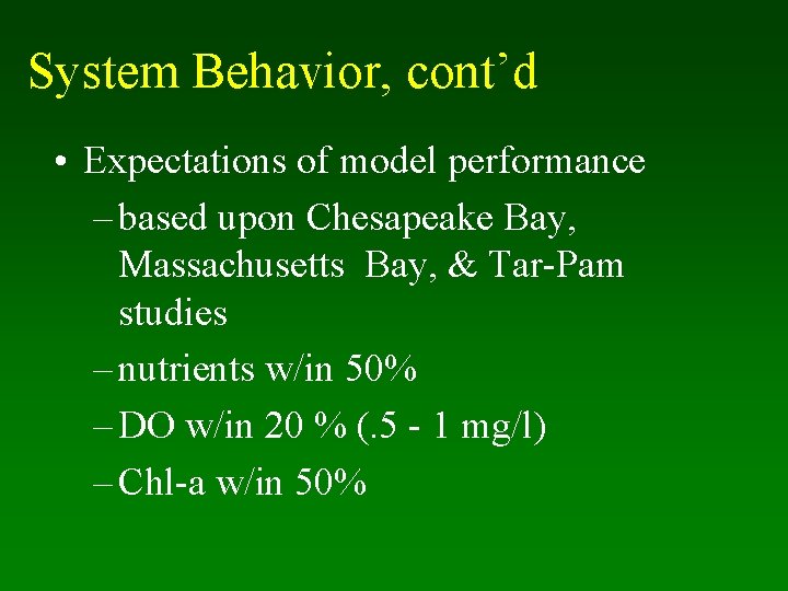
System Behavior, cont’d • Expectations of model performance – based upon Chesapeake Bay, Massachusetts Bay, & Tar-Pam studies – nutrients w/in 50% – DO w/in 20 % (. 5 - 1 mg/l) – Chl-a w/in 50%

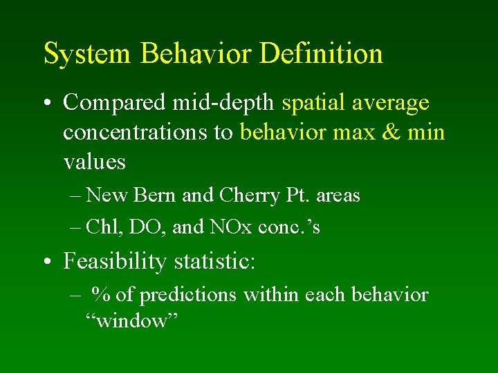
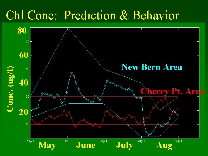
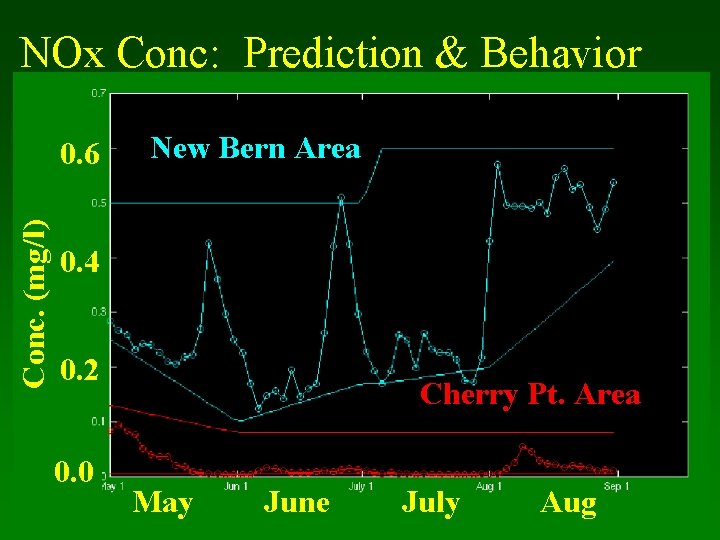
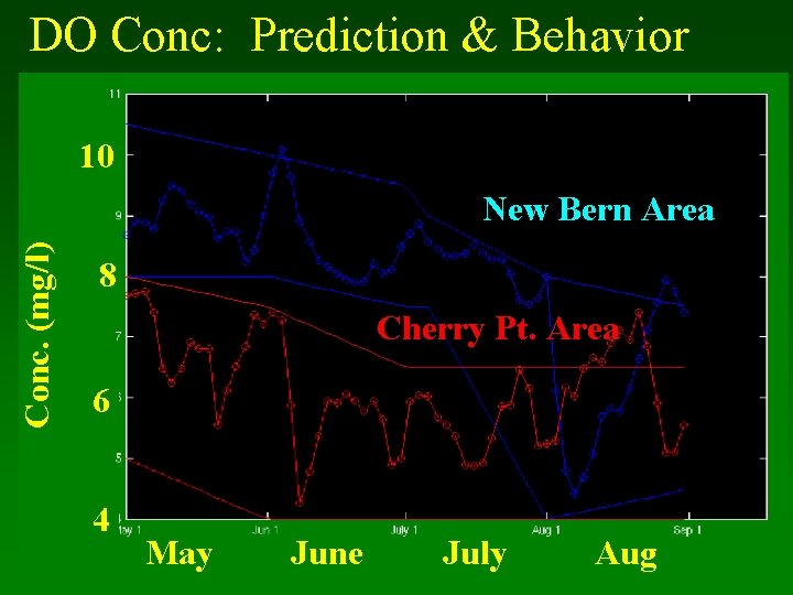
System Behavior Definition • Compared mid-depth spatial average concentrations to behavior max & min values – New Bern and Cherry Pt. areas – Chl, DO, and NOx conc. ’s • Feasibility statistic: – % of predictions within each behavior “window”

Chl Conc: Prediction & Behavior 80 Conc. (ug/l) 60 New Bern Area 40 Cherry Pt. Area 20 May June July Aug

NOx Conc: Prediction & Behavior Conc. (mg/l) 0. 6 New Bern Area 0. 4 0. 2 0. 0 Cherry Pt. Area May June July Aug

DO Conc: Prediction & Behavior 10 Conc. (mg/l) New Bern Area 8 Cherry Pt. Area 6 4 May June July Aug

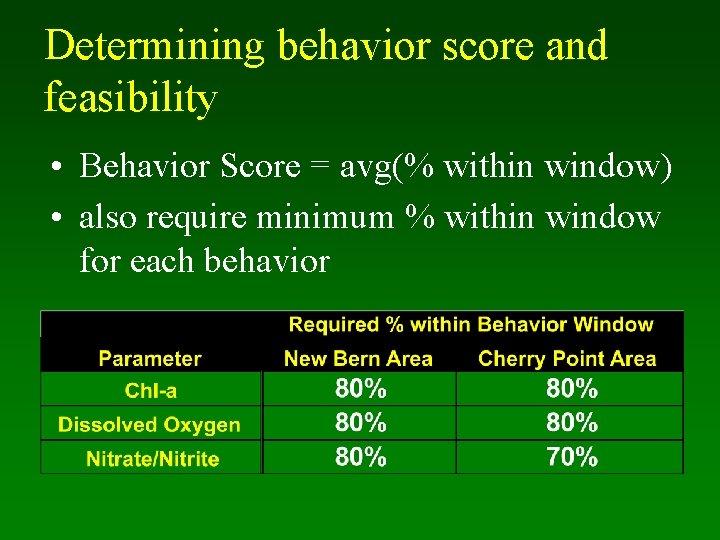
Determining behavior score and feasibility • Behavior Score = avg(% within window) • also require minimum % within window for each behavior

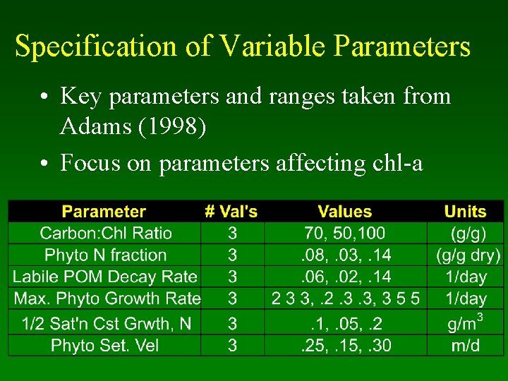
Specification of Variable Parameters • Key parameters and ranges taken from Adams (1998) • Focus on parameters affecting chl-a

Search for Feasible Parameter Vectors Preliminary Run (25 days) Accept = 31 Vectors #2 Final Run (120 days) Accept #1

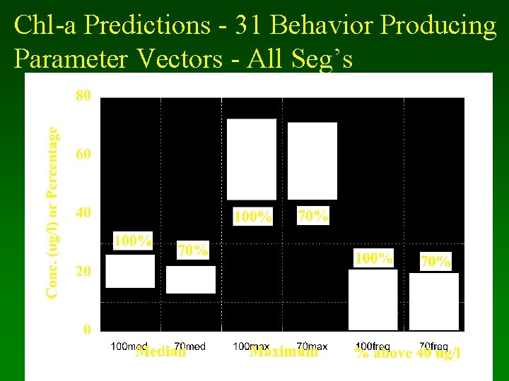
Chl-a Predictions - 31 Behavior Producing Parameter Vectors - All Seg’s

Chl-a Predictions - Cherry Point Segments

Percentage Reduction WQ Improvement: Chl Conc. & Exceedence Frequency Reductions

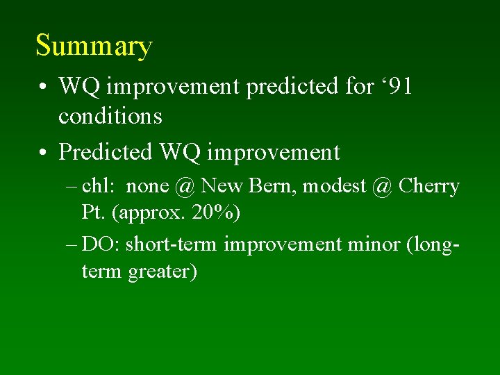
Summary • WQ improvement predicted for ‘ 91 conditions • Predicted WQ improvement – chl: none @ New Bern, modest @ Cherry Pt. (approx. 20%) – DO: short-term improvement minor (longterm greater)

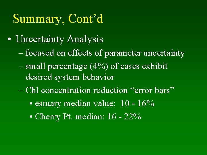
Summary, Cont’d • Uncertainty Analysis – focused on effects of parameter uncertainty – small percentage (4%) of cases exhibit desired system behavior – Chl concentration reduction “error bars” • estuary median value: 10 - 16% • Cherry Pt. median: 16 - 22%

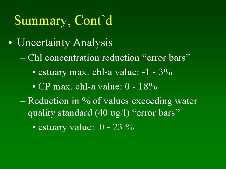
Summary, Cont’d • Uncertainty Analysis – Chl concentration reduction “error bars” • estuary max. chl-a value: -1 - 3% • CP max. chl-a value: 0 - 18% – Reduction in % of values exceeding water quality standard (40 ug/l) “error bars” • estuary value: 0 - 23 %

What’s left to do? • Repeat analysis for other years – 1997 simulations completed next month – 1998 simulations pending additional funding • Consider longer-term sediment “cleanup” – requires full calendar of monitoring data (e. g. 1998 data)

Looking Forward: Using MODMON monitoring for modeling • simulating different years helps to quantify uncertainty due to hydrologic variability • MODMON monitoring far superior to 1991 data set – much more frequent, many more stations, includes vertical profiles, includes more parameters, includes sed’s

MODMON monitoring data: 1997 vs. 1998 • 1997 features – similar hydrologically to 1991 – no downstream boundary conditions before June – dedicated downstream elevation monitor not installed – abundance of high-quality data available to aid calibration/ verification

Neuse Estuary Inflows

MODMON monitoring data: 1997 vs. 1998 • 1998 features – unusal year hydrologically with a significant fish kill – dedicated downstream elevation monitor installed – abundance of high-quality data available to aid calibration/ verification – full year of monitoring data will soon be available

More Things to Do • Investigate other reduction scenarios – % reduction larger in Spring, Summer – different % reductions (40%, 50%) • Conduct comprehensive error analysis – intelligent searches of parameter space – quantitative parameter filtering analysis to select variable parameters