MATH 175 NUMERICAL ANALYSIS II Lecturer Jomar Fajardo

MATH 175: NUMERICAL ANALYSIS II Lecturer: Jomar Fajardo Rabajante 2 nd Sem AY 2012 -2013 IMSP, UPLB

VARIABLE STEP-SIZE METHODS (ADAPTIVE) It is a good practice to change the step size for a solution that moves between periods of slow change and periods of fast change. One common variable step-size approach is using two solvers of different orders (embedded pairs).

VARIABLE STEP-SIZE METHODS Basic idea: 1. The user sets a tolerance error that must be met by each step. 2. The method is designed to reject the step and cut the step size (usually by half) if the tolerance error is exceeded. 3. If the tolerance error is met too well – say the error is 1/10 of the tolerance error – then the step size is increased (usually doubled). [We will not do number 3].

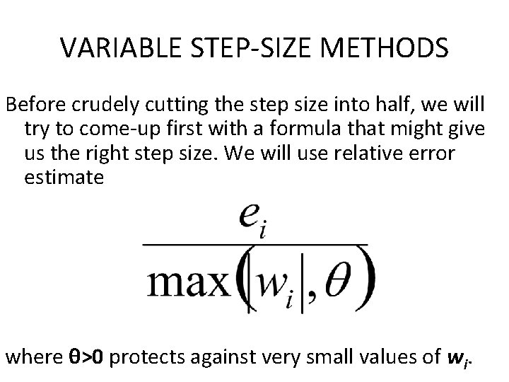
VARIABLE STEP-SIZE METHODS Before crudely cutting the step size into half, we will try to come-up first with a formula that might give us the right step size. We will use relative error estimate where θ>0 protects against very small values of wi.

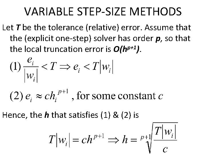
VARIABLE STEP-SIZE METHODS Let T be the tolerance (relative) error. Assume that the (explicit one-step) solver has order p, so that the local truncation error is O(hp+1). Hence, the h that satisfies (1) & (2) is

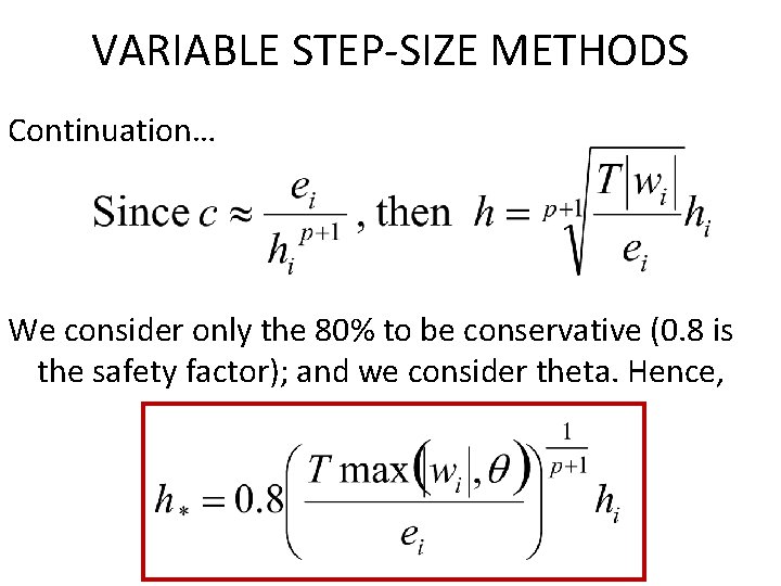
VARIABLE STEP-SIZE METHODS Continuation… We consider only the 80% to be conservative (0. 8 is the safety factor); and we consider theta. Hence,

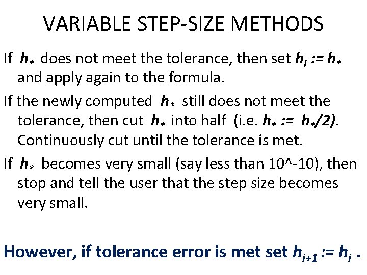
VARIABLE STEP-SIZE METHODS If h* does not meet the tolerance, then set hi : = h* and apply again to the formula. If the newly computed h* still does not meet the tolerance, then cut h* into half (i. e. h* : = h*/2). Continuously cut until the tolerance is met. If h* becomes very small (say less than 10^-10), then stop and tell the user that the step size becomes very small. However, if tolerance error is met set hi+1 : = hi.

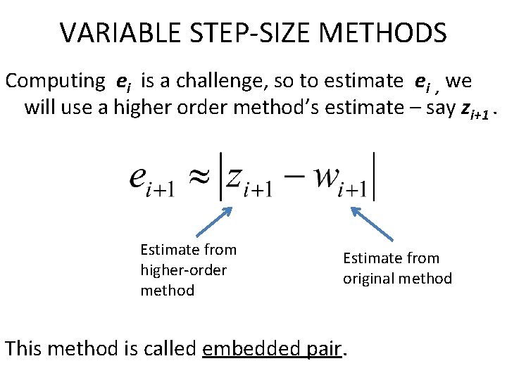
VARIABLE STEP-SIZE METHODS Computing ei is a challenge, so to estimate ei , we will use a higher order method’s estimate – say zi+1. Estimate from higher-order method Estimate from original method This method is called embedded pair.

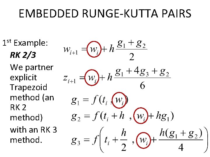
EMBEDDED RUNGE-KUTTA PAIRS 1 st Example: RK 2/3 We partner explicit Trapezoid method (an RK 2 method) with an RK 3 method.

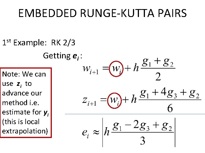
EMBEDDED RUNGE-KUTTA PAIRS 1 st Example: RK 2/3 Getting ei : Note: We can use zi to advance our method i. e. estimate for yi (this is local extrapolation)

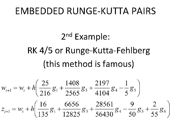
EMBEDDED RUNGE-KUTTA PAIRS 2 nd Example: RK 4/5 or Runge-Kutta-Fehlberg (this method is famous)

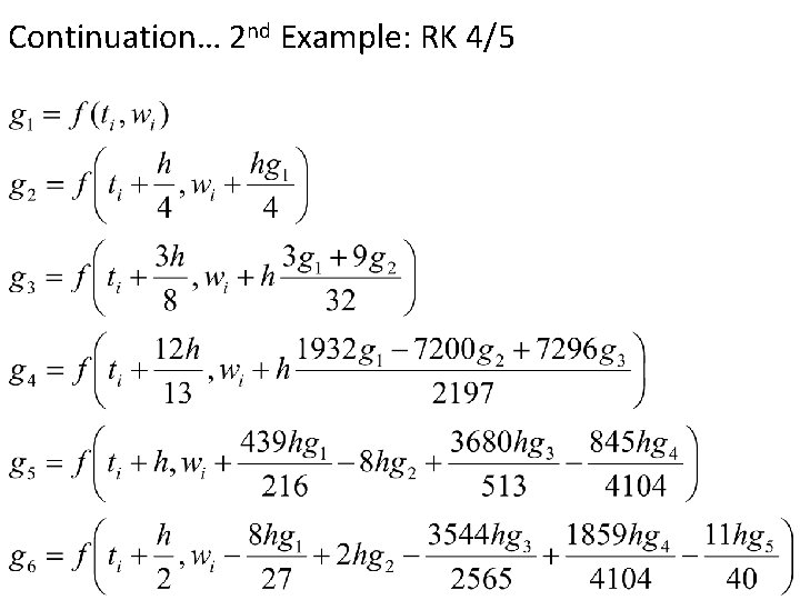
Continuation… 2 nd Example: RK 4/5

VARIABLE STEP-SIZE METHODS Other well-known methods: ØBogacki-Shampine 2/3 (ODE 23 in MATLAB) ØDormand-Prince 4/5 (ODE 45 in MATLAB) ØRKV 5/6 (Runge-Kutta-Verner) ØBulirsch-Stoer method You can also use Richardson’s extrapolation to improve the solutions. Note: There maybe other ways of computing h*.