HAPPY NEW YEAR MATH 175 NUMERICAL ANALYSIS II

HAPPY NEW YEAR!!! MATH 175: NUMERICAL ANALYSIS II CHAPTER 3: Differential Equations Lecturer: Jomar Fajardo Rabajante 2 nd Sem AY 2012 -2013 IMSP, UPLB

NUMERICAL SOLUTIONS TO DIFFERENTIAL EQUATIONS • Main Topic: Ordinary Differential Equations (Initial Value Problem) – Modeling – Numerical Solutions • Softwares: MS Excel, Sci. Lab, Berkeley Madonna • Optional Topics – Boundary Value Problem ODE – Partial Differential Equations – Stochastic Differential Equations

WHAT IS DE? Differential equations – the major interface of mathematics with the real world – are the main tool with which scientists make mathematical models of real systems. That is, differential equations have a central role in connecting the power of mathematics with the description of real phenomena. -John Hubbard, Cornell University

What is DE? Definition: A differential equation is an equation that contains derivatives of one or more dependent variables with respect to one or more independent variables. This is an extension of what you have learned in Math 30 series… MATH 151: Ordinary Differential Equations Math 152: Partial Differential Equations In Math 175: We will discuss how to solve problems that are not solvable in Math 151 and Math 152.

Examples:

Examples:

ODE and PDE • An ordinary differential equation contains only ordinary derivatives. Example: • A partial differential equation contains partial derivatives. Example:

Some concepts • Differential equations are for modeling continuous-time systems • Those discrete-time systems are modeled using difference equations (iterative equations, similar to our fixed-point iterations). Example:

Some concepts • Differential equations (DE) and difference equations are applied to model DYNAMICAL SYSTEMS – systems that change over time. • The order of a DE refers to the highest-order derivative that appears in the equation. Example:

Some concepts • Autonomous DEs – the variable t does not appear in the equation. Example: • Non-autonomous DEs – the variable t appears in the equation. Example:

Some concepts • Linear DE does not have transcendental and nonlinear dependent variables. Example of Linear DE: Example of Non-linear DE:

Very few physical systems are purely linear. But many nonlinear physical systems can be approximated by linear systems.

Let’s focus on ORDINARY DIFFERENTIAL EQUATIONS

SOLVING ODEs Example: The solution to the ODE dy/dt, also written as y’, is y(t) or y(t, y). • • • Obtaining an explicit formula: y(t) Obtaining an implicit formula: y(t, y) Obtaining a power series representation for y(t) Numerically approximating the solution y(t) or y(t, y) Sketching the geometric representation of y(t)

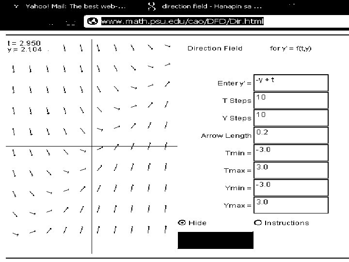
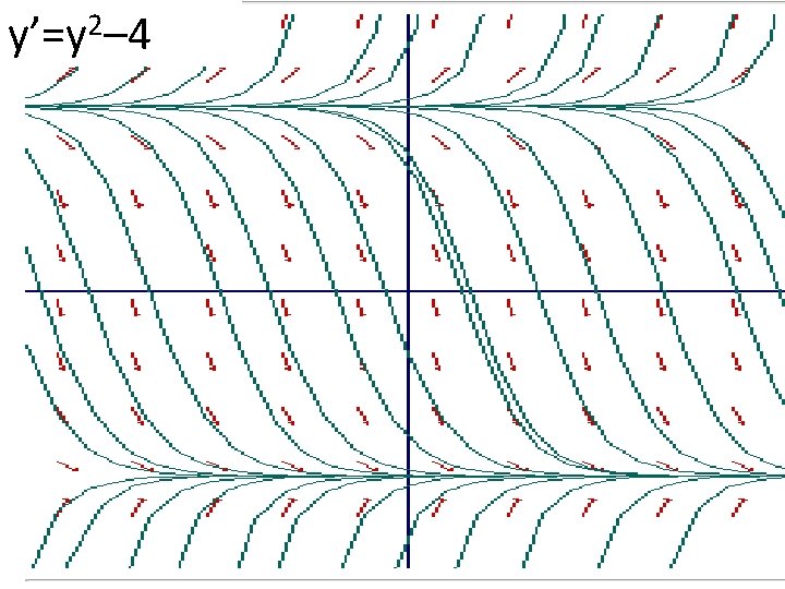
Geometric Representation FIRST-ORDER ODE • Direction Field/Slope Field Consider y’ = t – y Compute y’ (slopes) for every possible equally-spaced points (t, y). See http: //www. math. psu. edu/cao/DFD/Dir. html

Qualitative Analysis FIRST-ORDER ODE • Equilibria – solution that does not change over time i. e. dy/dt=0. • Stability of Equilibrium solution – Stable if solutions near it tend toward it as t ∞ – Unstable if solutions near it tend away from it as t ∞ – Saddle or semi-stable if stable on one side and unstable on the other. Note: A good practice when studying DEs is to investigate first its qualitative properties. Many physical systems modeled by DEs “spend most of their time at or near equilibrium states. ”

INITIAL VALUE PROBLEM The combination of a differential equation and an initial condition is called an initial-value problem. Example: (You do not need +c when dealing with IVP)