Management Science Goh Chapter 1 Introduction Origin of

Management Science (Goh) Chapter 1: Introduction Ø Ø Ø Ø Origin of Management Science Problem Solving and Decision Making Problem Analysis and Decision Making Qualitative vs. Quantitative Analysis Model Development Deterministic vs. Stoochastic Models of Cost, Revenue, and Profit Quantitative Methods in Practice Slide 1

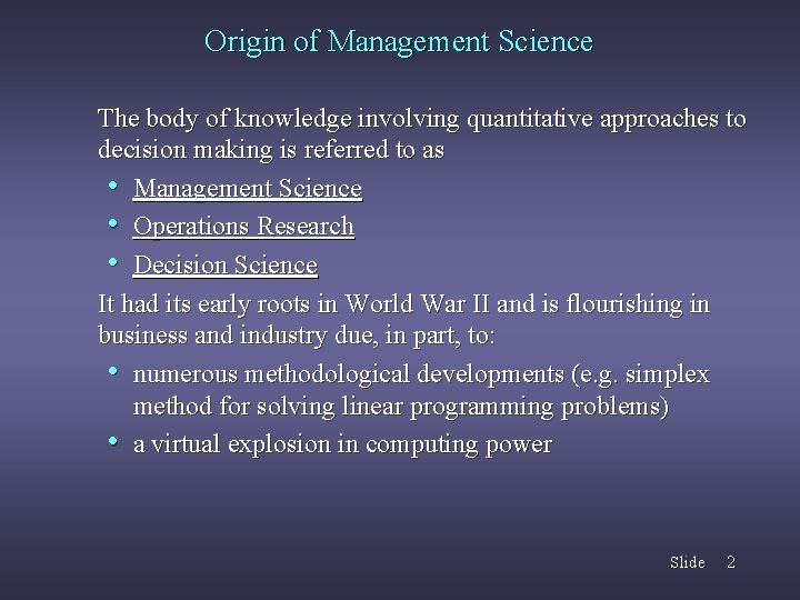
Origin of Management Science The body of knowledge involving quantitative approaches to decision making is referred to as • Management Science • Operations Research • Decision Science It had its early roots in World War II and is flourishing in business and industry due, in part, to: • numerous methodological developments (e. g. simplex method for solving linear programming problems) • a virtual explosion in computing power Slide 2

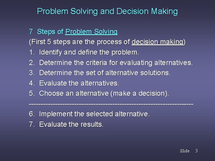
Problem Solving and Decision Making 7 Steps of Problem Solving (First 5 steps are the process of decision making) 1. Identify and define the problem. 2. Determine the criteria for evaluating alternatives. 3. Determine the set of alternative solutions. 4. Evaluate the alternatives. 5. Choose an alternative (make a decision). ----------------------------------6. Implement the selected alternative. 7. Evaluate the results. Slide 3

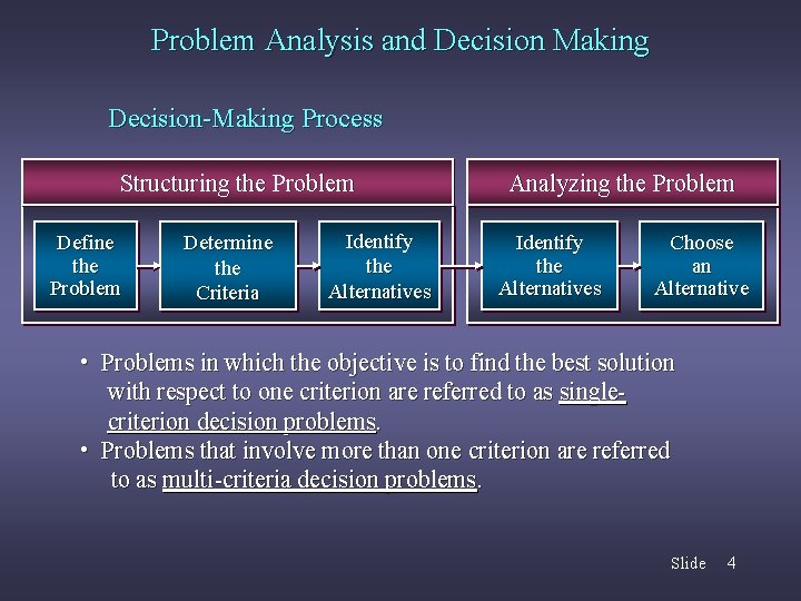
Problem Analysis and Decision Making Decision-Making Process Structuring the Problem Define the Problem Determine the Criteria Identify the Alternatives Analyzing the Problem Identify the Alternatives Choose an Alternative • Problems in which the objective is to find the best solution with respect to one criterion are referred to as singlecriterion decision problems. • Problems that involve more than one criterion are referred to as multi-criteria decision problems. Slide 4

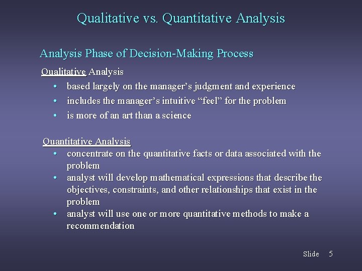
Qualitative vs. Quantitative Analysis Phase of Decision-Making Process Qualitative Analysis • based largely on the manager’s judgment and experience • includes the manager’s intuitive “feel” for the problem • is more of an art than a science Quantitative Analysis • concentrate on the quantitative facts or data associated with the problem • analyst will develop mathematical expressions that describe the objectives, constraints, and other relationships that exist in the problem • analyst will use one or more quantitative methods to make a recommendation Slide 5

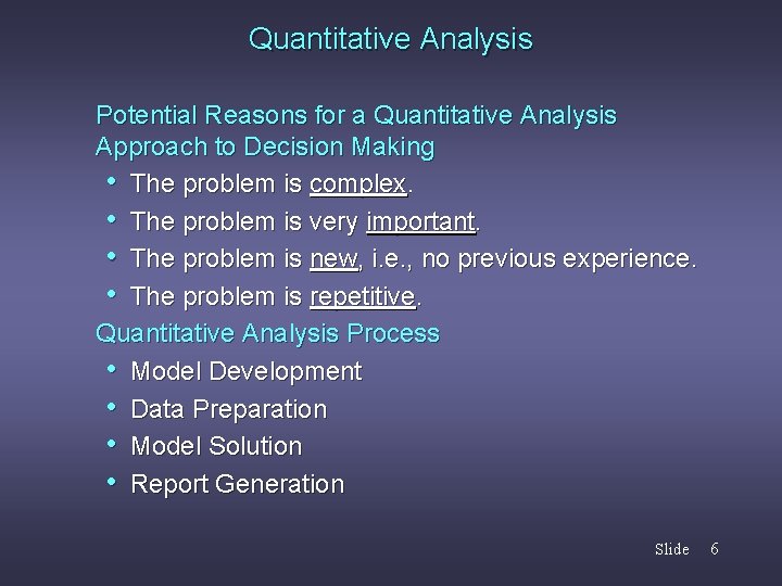
Quantitative Analysis Potential Reasons for a Quantitative Analysis Approach to Decision Making • The problem is complex. • The problem is very important. • The problem is new, i. e. , no previous experience. • The problem is repetitive. Quantitative Analysis Process • Model Development • Data Preparation • Model Solution • Report Generation Slide 6

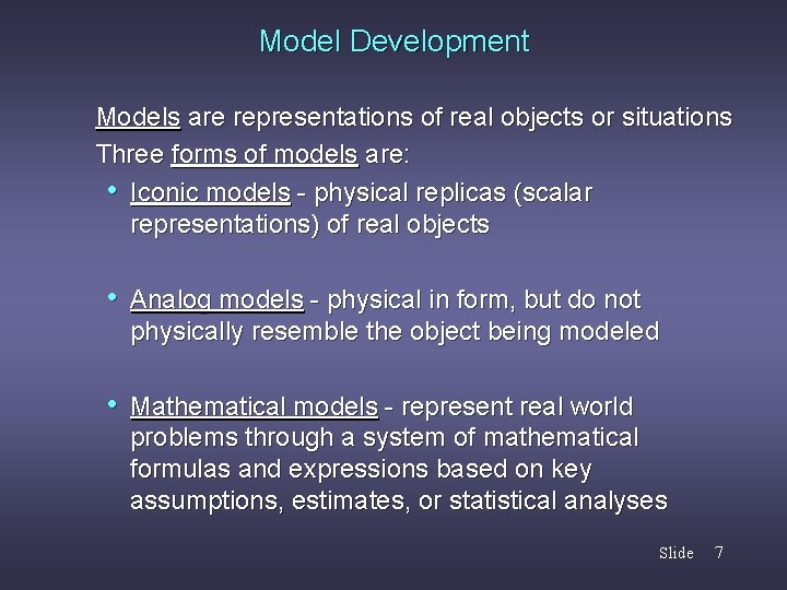
Model Development Models are representations of real objects or situations Three forms of models are: • Iconic models - physical replicas (scalar representations) of real objects • Analog models - physical in form, but do not physically resemble the object being modeled • Mathematical models - represent real world problems through a system of mathematical formulas and expressions based on key assumptions, estimates, or statistical analyses Slide 7

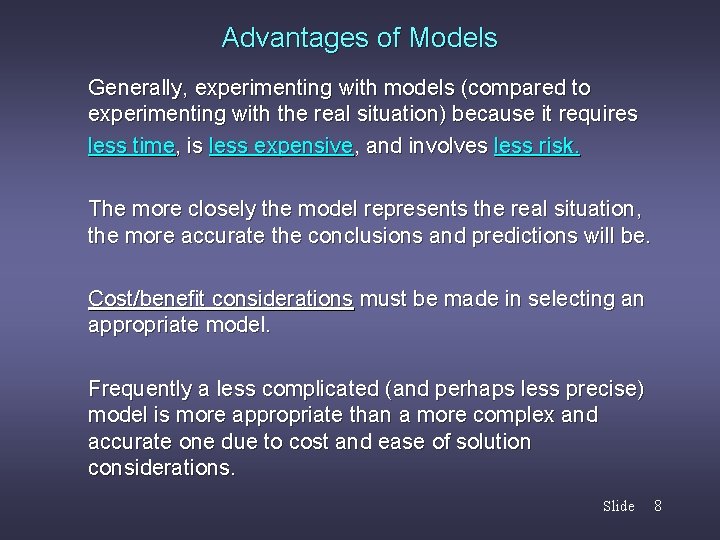
Advantages of Models Generally, experimenting with models (compared to experimenting with the real situation) because it requires less time, is less expensive, and involves less risk. The more closely the model represents the real situation, the more accurate the conclusions and predictions will be. Cost/benefit considerations must be made in selecting an appropriate model. Frequently a less complicated (and perhaps less precise) model is more appropriate than a more complex and accurate one due to cost and ease of solution considerations. Slide 8

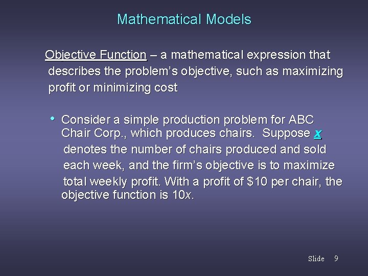
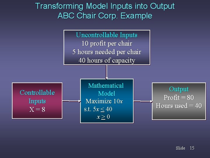
Mathematical Models Objective Function – a mathematical expression that describes the problem’s objective, such as maximizing profit or minimizing cost • Consider a simple production problem for ABC Chair Corp. , which produces chairs. Suppose x denotes the number of chairs produced and sold each week, and the firm’s objective is to maximize total weekly profit. With a profit of $10 per chair, the objective function is 10 x. Slide 9

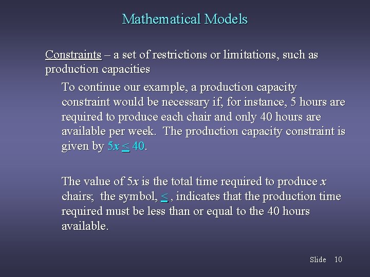
Mathematical Models Constraints – a set of restrictions or limitations, such as production capacities To continue our example, a production capacity constraint would be necessary if, for instance, 5 hours are required to produce each chair and only 40 hours are available per week. The production capacity constraint is given by 5 x < 40. The value of 5 x is the total time required to produce x chairs; the symbol, < , indicates that the production time required must be less than or equal to the 40 hours available. Slide 10

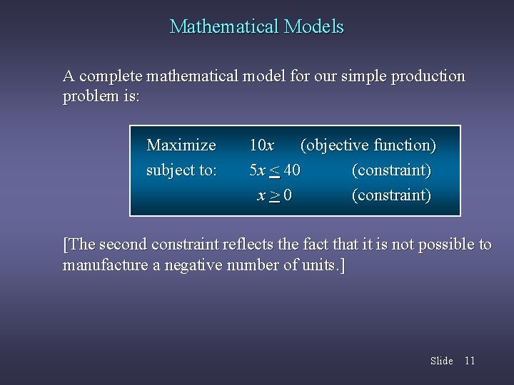
Mathematical Models A complete mathematical model for our simple production problem is: Maximize subject to: 10 x (objective function) 5 x < 40 (constraint) x>0 (constraint) [The second constraint reflects the fact that it is not possible to manufacture a negative number of units. ] Slide 11

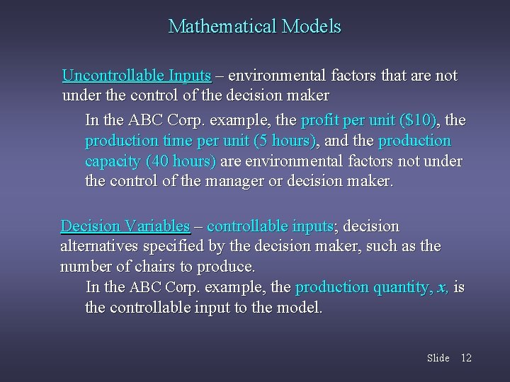
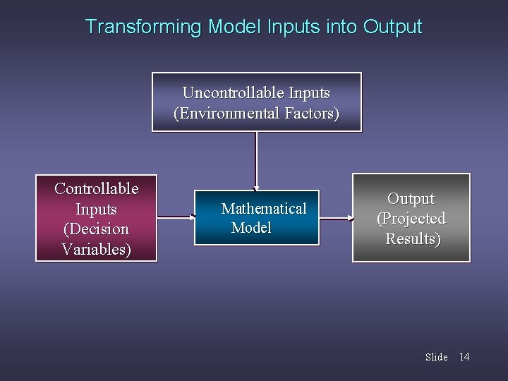
Mathematical Models Uncontrollable Inputs – environmental factors that are not under the control of the decision maker In the ABC Corp. example, the profit per unit ($10), the production time per unit (5 hours), and the production capacity (40 hours) are environmental factors not under the control of the manager or decision maker. Decision Variables – controllable inputs; decision alternatives specified by the decision maker, such as the number of chairs to produce. In the ABC Corp. example, the production quantity, x, is the controllable input to the model. Slide 12

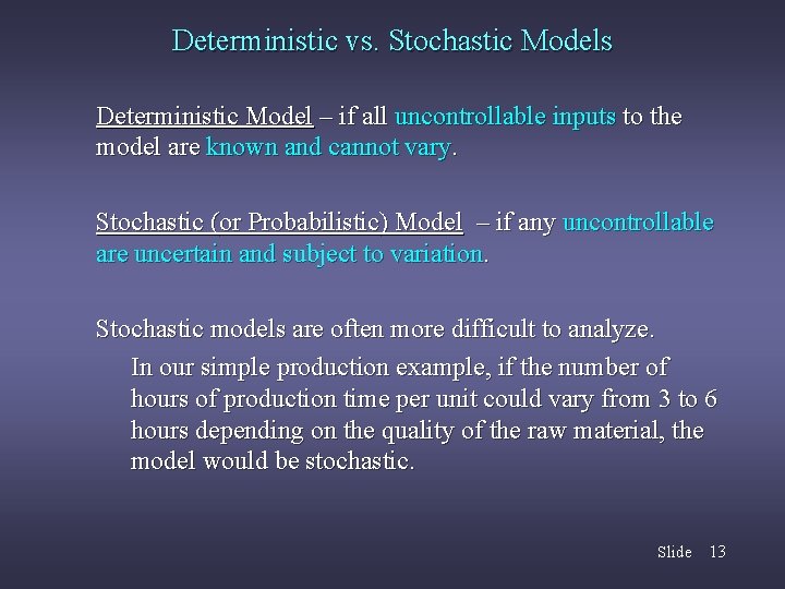
Deterministic vs. Stochastic Models Deterministic Model – if all uncontrollable inputs to the model are known and cannot vary. Stochastic (or Probabilistic) Model – if any uncontrollable are uncertain and subject to variation. Stochastic models are often more difficult to analyze. In our simple production example, if the number of hours of production time per unit could vary from 3 to 6 hours depending on the quality of the raw material, the model would be stochastic. Slide 13

Transforming Model Inputs into Output Uncontrollable Inputs (Environmental Factors) Controllable Inputs (Decision Variables) Mathematical Model Output (Projected Results) Slide 14

Transforming Model Inputs into Output ABC Chair Corp. Example Uncontrollable Inputs 10 profit per chair 5 hours needed per chair 40 hours of capacity Controllable Inputs X=8 Mathematical Model Maximize 10 x s. t. 5 x < 40 x>0 Output Profit = 80 Hours used = 40 Slide 15

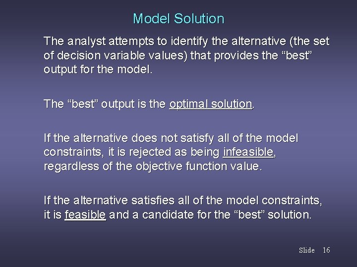
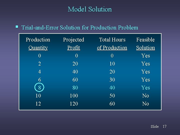
Model Solution The analyst attempts to identify the alternative (the set of decision variable values) that provides the “best” output for the model. The “best” output is the optimal solution. If the alternative does not satisfy all of the model constraints, it is rejected as being infeasible, regardless of the objective function value. If the alternative satisfies all of the model constraints, it is feasible and a candidate for the “best” solution. Slide 16

Model Solution § Trial-and-Error Solution for Production Problem Production Quantity 0 2 4 6 8 10 12 Projected Profit 0 20 40 60 80 100 120 Total Hours of Production 0 10 20 30 40 50 60 Feasible Solution Yes Yes Yes No No Slide 17

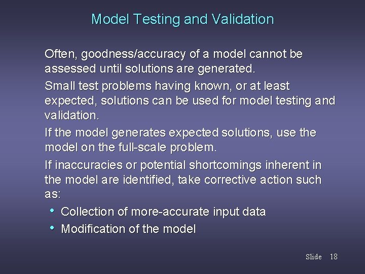
Model Testing and Validation Often, goodness/accuracy of a model cannot be assessed until solutions are generated. Small test problems having known, or at least expected, solutions can be used for model testing and validation. If the model generates expected solutions, use the model on the full-scale problem. If inaccuracies or potential shortcomings inherent in the model are identified, take corrective action such as: • Collection of more-accurate input data • Modification of the model Slide 18

Report Generation A managerial report, based on the results of the model, should be prepared. The report should be easily understood by the decision maker. The report should include: • the recommended decision • other pertinent information about the results (for example, how sensitive the model solution is to the assumptions and data used in the model) Slide 19

Implementation and Follow-Up Successful implementation of model results is of critical importance. Secure as much user involvement as possible throughout the modeling process. Continue to monitor the contribution of the model. It might be necessary to refine or expand the model. Slide 20

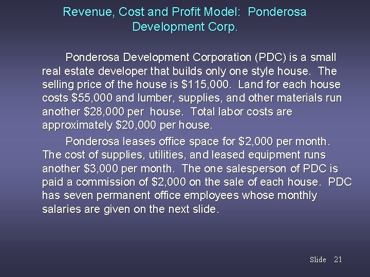
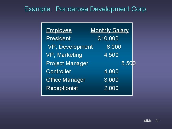
Revenue, Cost and Profit Model: Ponderosa Development Corporation (PDC) is a small real estate developer that builds only one style house. The selling price of the house is $115, 000. Land for each house costs $55, 000 and lumber, supplies, and other materials run another $28, 000 per house. Total labor costs are approximately $20, 000 per house. Ponderosa leases office space for $2, 000 per month. The cost of supplies, utilities, and leased equipment runs another $3, 000 per month. The one salesperson of PDC is paid a commission of $2, 000 on the sale of each house. PDC has seven permanent office employees whose monthly salaries are given on the next slide. Slide 21

Example: Ponderosa Development Corp. Employee Monthly Salary President $10, 000 VP, Development 6, 000 VP, Marketing 4, 500 Project Manager 5, 500 Controller 4, 000 Office Manager 3, 000 Receptionist 2, 000 Slide 22

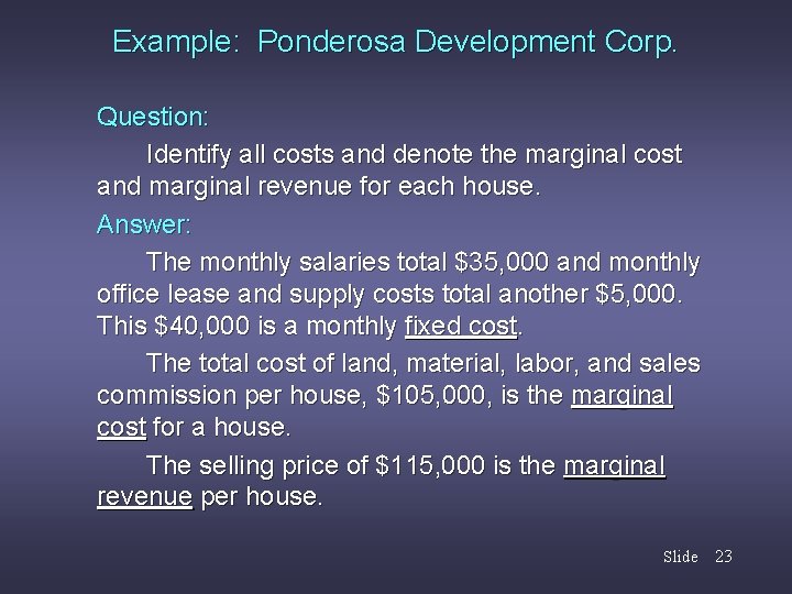
Example: Ponderosa Development Corp. Question: Identify all costs and denote the marginal cost and marginal revenue for each house. Answer: The monthly salaries total $35, 000 and monthly office lease and supply costs total another $5, 000. This $40, 000 is a monthly fixed cost. The total cost of land, material, labor, and sales commission per house, $105, 000, is the marginal cost for a house. The selling price of $115, 000 is the marginal revenue per house. Slide 23

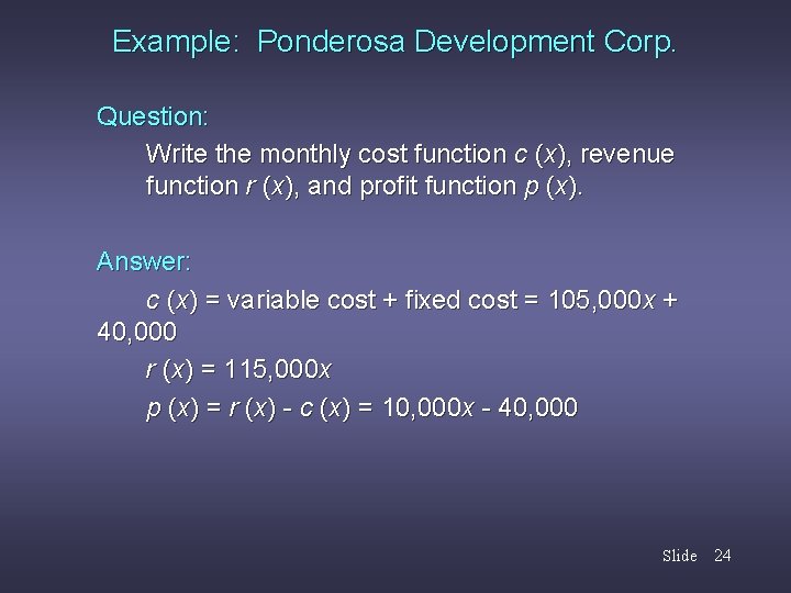
Example: Ponderosa Development Corp. Question: Write the monthly cost function c (x), revenue function r (x), and profit function p (x). Answer: c (x) = variable cost + fixed cost = 105, 000 x + 40, 000 r (x) = 115, 000 x p (x) = r (x) - c (x) = 10, 000 x - 40, 000 Slide 24

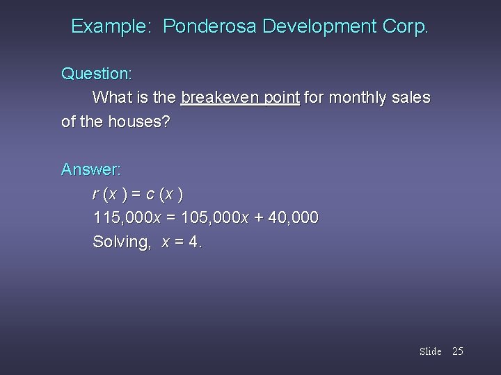
Example: Ponderosa Development Corp. Question: What is the breakeven point for monthly sales of the houses? Answer: r (x ) = c (x ) 115, 000 x = 105, 000 x + 40, 000 Solving, x = 4. Slide 25

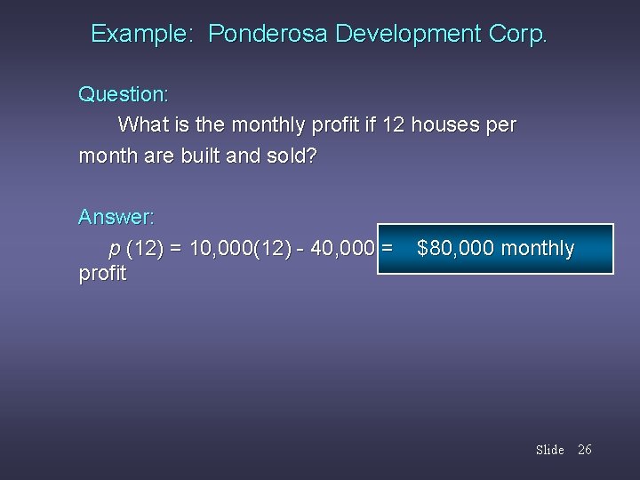
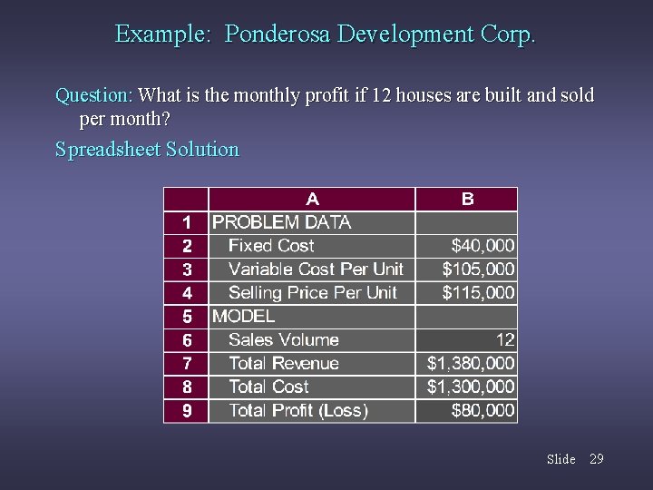
Example: Ponderosa Development Corp. Question: What is the monthly profit if 12 houses per month are built and sold? Answer: p (12) = 10, 000(12) - 40, 000 = profit $80, 000 monthly Slide 26

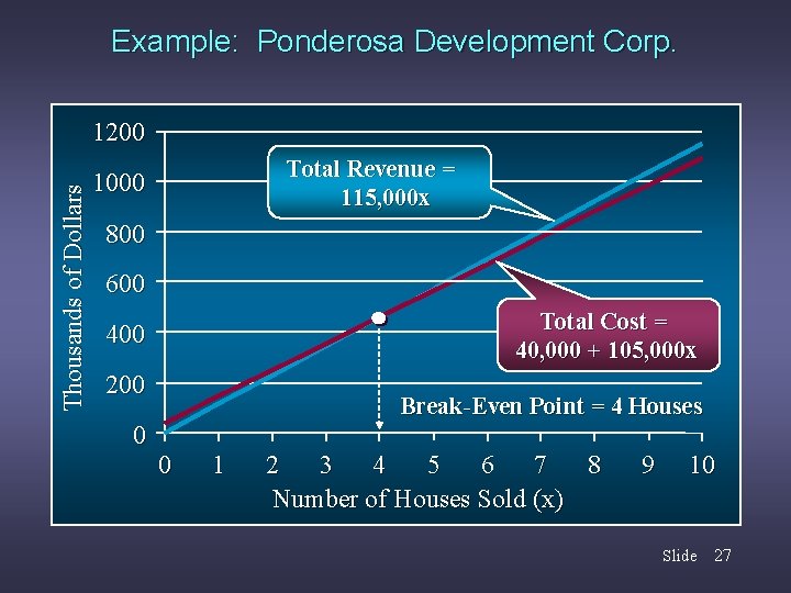
Example: Ponderosa Development Corp. Thousands of Dollars 1200 Total Revenue = 115, 000 x 1000 800 600 Total Cost = 40, 000 + 105, 000 x 400 200 Break-Even Point = 4 Houses 0 0 1 2 3 4 5 6 7 8 Number of Houses Sold (x) 9 10 Slide 27

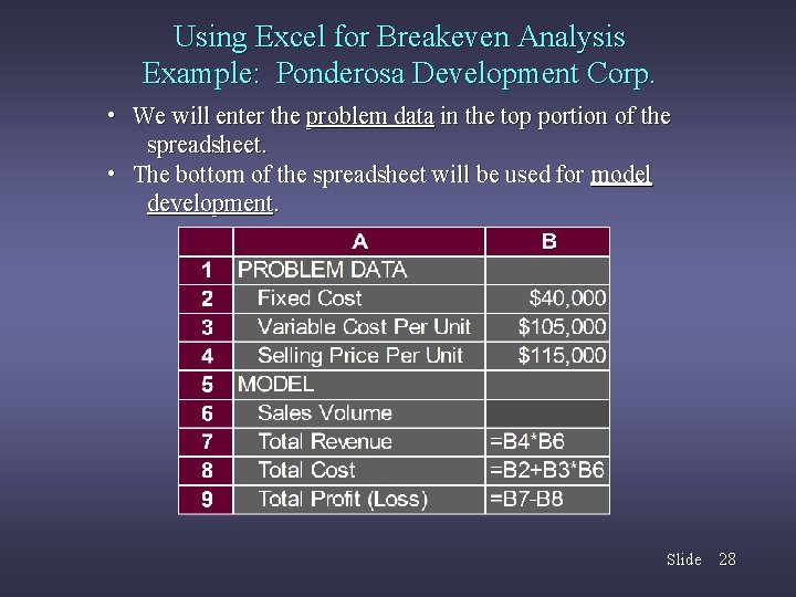
Using Excel for Breakeven Analysis Example: Ponderosa Development Corp. • We will enter the problem data in the top portion of the spreadsheet. • The bottom of the spreadsheet will be used for model development. Slide 28

Example: Ponderosa Development Corp. Question: What is the monthly profit if 12 houses are built and sold per month? Spreadsheet Solution Slide 29

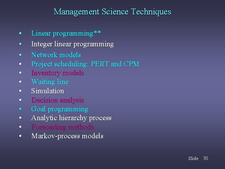
Management Science Techniques • • • Linear programming** Integer linear programming Network models Project scheduling: PERT and CPM Inventory models Waiting line Simulation Decision analysis Goal programming Analytic hierarchy process Forecasting methods. Markov-process models Slide 30