Management of Economic Exposure Chapter Nine Copyright 2012

Management of Economic Exposure Chapter Nine Copyright © 2012 by the Mc. Graw-Hill Companies, Inc. All rights reserved.

Chapter Outline § § § How to Measure Economic Exposure Operating Exposure: Definition An Illustration of Operating Exposure Determinants of Operating Exposure Managing Operating Exposure 9 -2

Economic Exposure § Changes in exchange rates can affect not only firms that are directly engaged in international trade but also purely domestic firms. § If the domestic firm’s products compete with imported goods, then their competitive position is affected by the strength or weakness of the local currency. 9 -3

Economic Exposure § Consider a U. S. bicycle manufacturer who sources, produces, and sells only in the U. S. § Since the firm’s product competes against imported bicycles, it is subject to foreign exchange exposure. § Their customers are comparing the cost and features of the domestic bicycle against Japanese, British, and Italian bicycles. 9 -4

Economic Exposure § Exchange rate risk is applied to the firm’s competitive position. § Any anticipated changes in the exchange rates would already have been discounted and reflected in the firm’s value. § Economic exposure can be defined as the extent to which the value of the firm would be affected by unanticipated changes in exchange rates. 9 -5

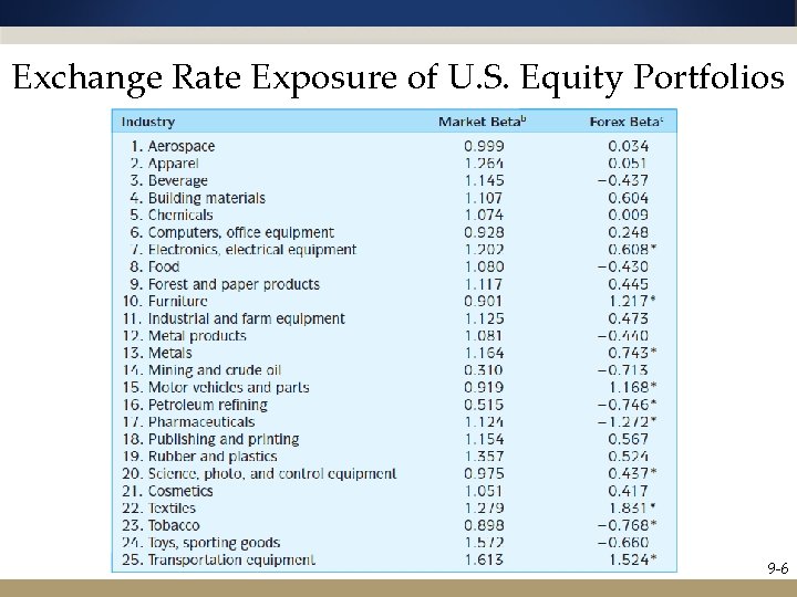
Exchange Rate Exposure of U. S. Equity Portfolios 9 -6

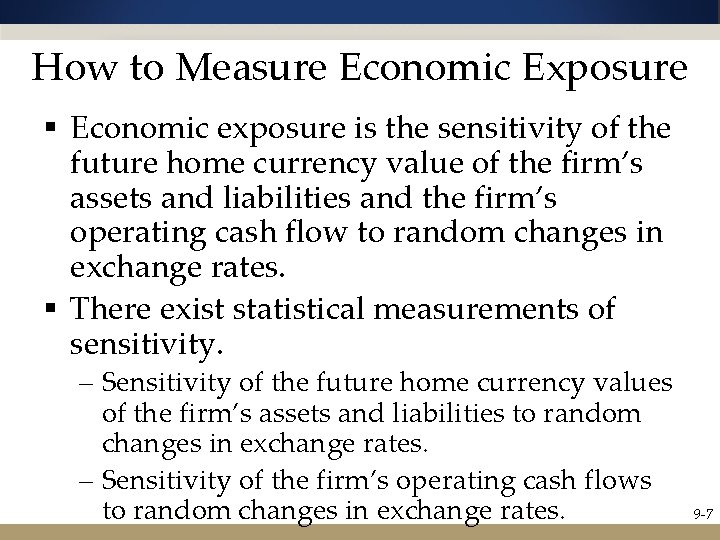
How to Measure Economic Exposure § Economic exposure is the sensitivity of the future home currency value of the firm’s assets and liabilities and the firm’s operating cash flow to random changes in exchange rates. § There exist statistical measurements of sensitivity. – Sensitivity of the future home currency values of the firm’s assets and liabilities to random changes in exchange rates. – Sensitivity of the firm’s operating cash flows to random changes in exchange rates. 9 -7

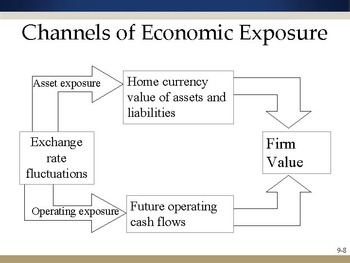
Channels of Economic Exposure Asset exposure Home currency value of assets and liabilities Exchange rate fluctuations Firm Value Operating exposure Future operating cash flows 9 -8

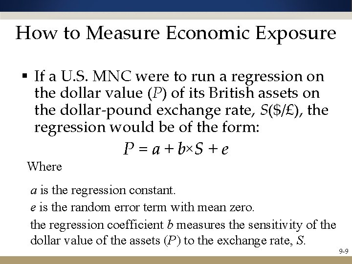
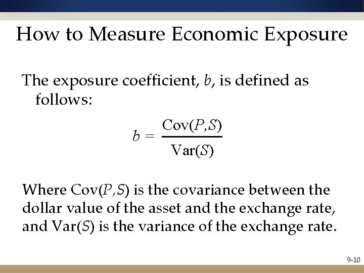
How to Measure Economic Exposure § If a U. S. MNC were to run a regression on the dollar value (P) of its British assets on the dollar-pound exchange rate, S($/£), the regression would be of the form: Where P = a + b×S + e a is the regression constant. e is the random error term with mean zero. the regression coefficient b measures the sensitivity of the dollar value of the assets (P) to the exchange rate, S. 9 -9

How to Measure Economic Exposure The exposure coefficient, b, is defined as follows: b= Cov(P, S) Var(S) Where Cov(P, S) is the covariance between the dollar value of the asset and the exchange rate, and Var(S) is the variance of the exchange rate. 9 -10

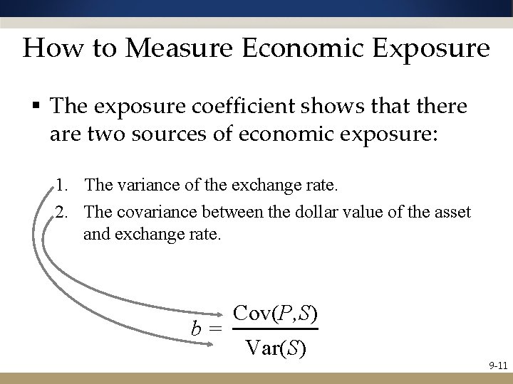
How to Measure Economic Exposure § The exposure coefficient shows that there are two sources of economic exposure: 1. The variance of the exchange rate. 2. The covariance between the dollar value of the asset and exchange rate. b= Cov(P, S) Var(S) 9 -11

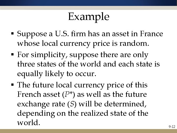
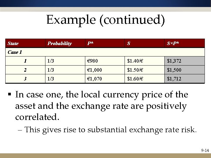
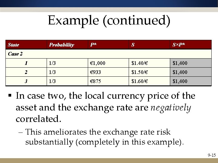
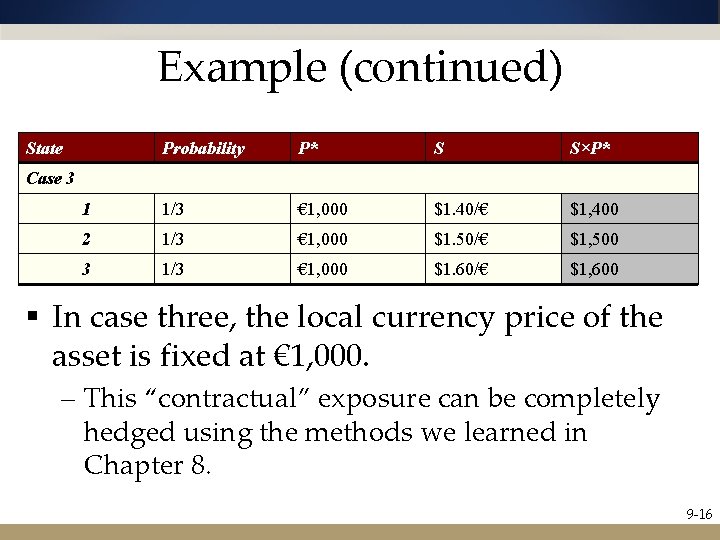
Example § Suppose a U. S. firm has an asset in France whose local currency price is random. § For simplicity, suppose there are only three states of the world and each state is equally likely to occur. § The future local currency price of this French asset (P*) as well as the future exchange rate (S) will be determined, depending on the realized state of the world. 9 -12

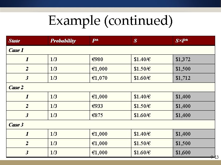
Example (continued) State Probability P* S S×P* 1 1/3 € 980 $1. 40/€ $1, 372 2 1/3 € 1, 000 $1. 50/€ $1, 500 3 1/3 € 1, 070 $1. 60/€ $1, 712 1 1/3 € 1, 000 $1. 40/€ $1, 400 2 1/3 € 933 $1. 50/€ $1, 400 3 1/3 € 875 $1. 60/€ $1, 400 1 1/3 € 1, 000 $1. 40/€ $1, 400 2 1/3 € 1, 000 $1. 50/€ $1, 500 3 1/3 € 1, 000 $1. 60/€ $1, 600 Case 1 Case 2 Case 3 9 -13

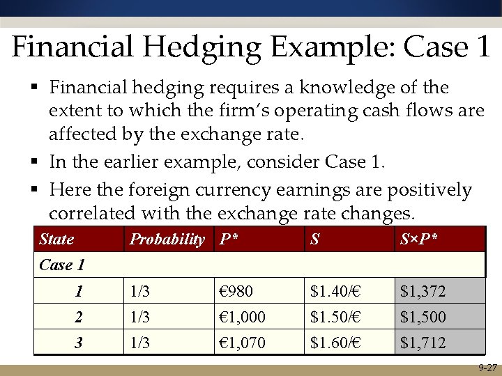
Example (continued) State Probability P* S S×P* 1 1/3 € 980 $1. 40/€ $1, 372 2 1/3 € 1, 000 $1. 50/€ $1, 500 3 1/3 € 1, 070 $1. 60/€ $1, 712 Case 1 § In case one, the local currency price of the asset and the exchange rate are positively correlated. – This gives rise to substantial exchange rate risk. 9 -14

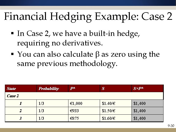
Example (continued) State Probability P* S S×P* 1 1/3 € 1, 000 $1. 40/€ $1, 400 2 1/3 € 933 $1. 50/€ $1, 400 3 1/3 € 875 $1. 60/€ $1, 400 Case 2 § In case two, the local currency price of the asset and the exchange rate are negatively correlated. – This ameliorates the exchange rate risk substantially (completely in this example). 9 -15

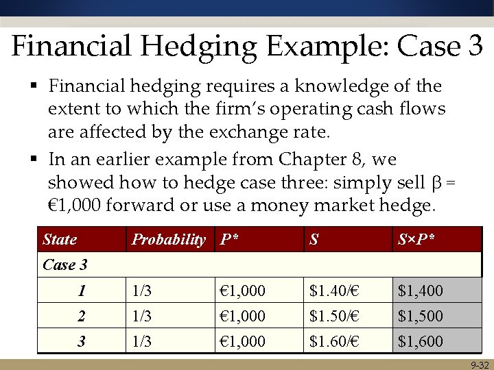
Example (continued) State Probability P* S S×P* 1 1/3 € 1, 000 $1. 40/€ $1, 400 2 1/3 € 1, 000 $1. 50/€ $1, 500 3 1/3 € 1, 000 $1. 60/€ $1, 600 Case 3 § In case three, the local currency price of the asset is fixed at € 1, 000. – This “contractual” exposure can be completely hedged using the methods we learned in Chapter 8. 9 -16

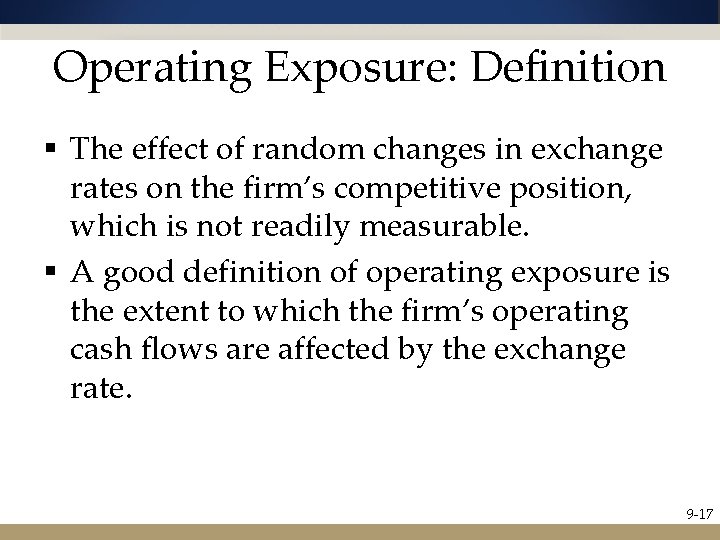
Operating Exposure: Definition § The effect of random changes in exchange rates on the firm’s competitive position, which is not readily measurable. § A good definition of operating exposure is the extent to which the firm’s operating cash flows are affected by the exchange rate. 9 -17

An Illustration of Operating Exposure § There was an enormous shortage in the shipping market from Asia due to the Asian currency crisis. § This affected not only the shipping companies, who enjoyed “boom times, ” but also retailers, who experienced increased costs and delays. 9 -18

An Illustration of Operating Exposure § Note that the exposure for the retailers has two components. – The competitive effect: • Difficulties and increased costs of shipping – The conversion effect: • Lower dollar prices of imports due to foreign currency exchange rate depreciation. 9 -19

Determinants of Operating Exposure § § Recall that operating exposure cannot be readily determined from the firm’s accounting statements as can transaction exposure. The firm’s operating exposure is determined by: – The market structure of inputs and products; how – competitive or how monopolistic the markets facing the firm are. The firm’s ability to adjust its markets, product mix, and sourcing in response to exchange rate changes. 9 -20

Managing Operating Exposure § § § Selecting Low Cost Production Sites Flexible Sourcing Policy Diversification of the Market R&D and Product Differentiation Financial Hedging 9 -21

Selecting Low Cost Production Sites § A firm may wish to diversify the location of its production sites to mitigate the effect of exchange rate movements. § For example, Honda built North American factories in response to a strong yen, but later found itself importing more cars from Japan due to a weak yen. 9 -22

Flexible Sourcing Policy § Sourcing does not apply only to components, but also to “guest workers. ” § For example, Japan Air Lines hired foreign crews to remain competitive in international routes in the face of a strong yen, but later contemplated a reverse strategy in the face of a weak yen and rising domestic unemployment. 9 -23

Diversification of the Market § Selling in multiple markets to take advantage of economies of scale and diversification of exchange rate risk. 9 -24

R&D and Product Differentiation § Successful research and development (R&D) allows for: – Cost-cutting – Enhanced productivity – Product differentiation § Successful product differentiation gives the firm less elastic demand—which may translate into less exchange rate risk. 9 -25

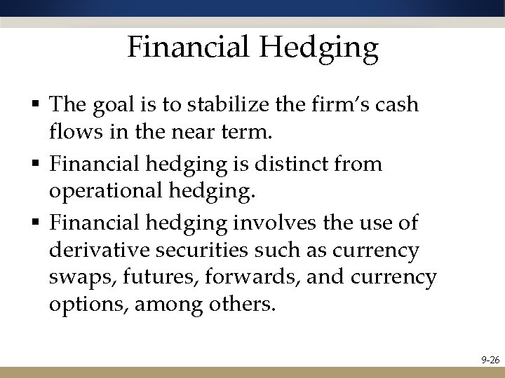
Financial Hedging § The goal is to stabilize the firm’s cash flows in the near term. § Financial hedging is distinct from operational hedging. § Financial hedging involves the use of derivative securities such as currency swaps, futures, forwards, and currency options, among others. 9 -26

Financial Hedging Example: Case 1 § Financial hedging requires a knowledge of the extent to which the firm’s operating cash flows are affected by the exchange rate. § In the earlier example, consider Case 1. § Here the foreign currency earnings are positively correlated with the exchange rate changes. State Probability P* S S×P* 1 1/3 € 980 $1. 40/€ $1, 372 2 1/3 € 1, 000 $1. 50/€ $1, 500 3 1/3 € 1, 070 $1. 60/€ $1, 712 Case 1 9 -27

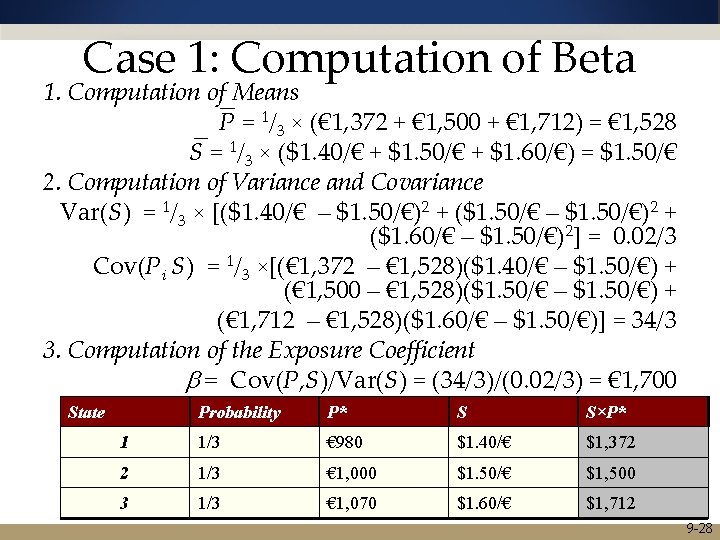
Case 1: Computation of Beta 1. Computation of Means P = 1/3 × (€ 1, 372 + € 1, 500 + € 1, 712) = € 1, 528 S = 1/3 × ($1. 40/€ + $1. 50/€ + $1. 60/€) = $1. 50/€ 2. Computation of Variance and Covariance Var(S) = 1/3 × [($1. 40/€ – $1. 50/€)2 + ($1. 50/€ – $1. 50/€)2 + ($1. 60/€ – $1. 50/€)2] = 0. 02/3 Cov(Pi S) = 1/3 ×[(€ 1, 372 – € 1, 528)($1. 40/€ – $1. 50/€) + (€ 1, 500 – € 1, 528)($1. 50/€ – $1. 50/€) + (€ 1, 712 – € 1, 528)($1. 60/€ – $1. 50/€)] = 34/3 3. Computation of the Exposure Coefficient b = Cov(P, S)/Var(S) = (34/3)/(0. 02/3) = € 1, 700 State Probability P* S S×P* 1 1/3 € 980 $1. 40/€ $1, 372 2 1/3 € 1, 000 $1. 50/€ $1, 500 3 1/3 € 1, 070 $1. 60/€ $1, 712 9 -28

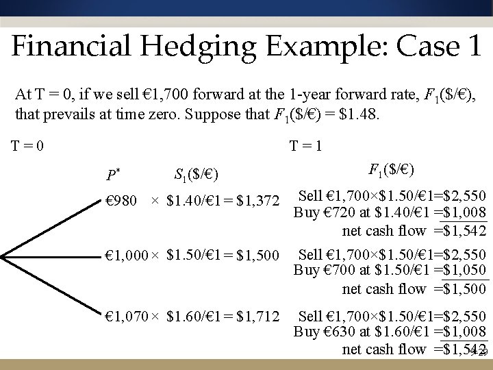
Financial Hedging Example: Case 1 At T = 0, if we sell € 1, 700 forward at the 1 -year forward rate, F 1($/€), that prevails at time zero. Suppose that F 1($/€) = $1. 48. T=0 T=1 S 1($/€) F 1($/€) € 980 × $1. 40/€ 1 = $1, 372 Sell € 1, 700×$1. 50/€ 1=$2, 550 Buy € 720 at $1. 40/€ 1 =$1, 008 net cash flow =$1, 542 € 1, 000 × $1. 50/€ 1 = $1, 500 Sell € 1, 700×$1. 50/€ 1=$2, 550 Buy € 700 at $1. 50/€ 1 =$1, 050 net cash flow =$1, 500 € 1, 070 × $1. 60/€ 1 = $1, 712 Sell € 1, 700×$1. 50/€ 1=$2, 550 Buy € 630 at $1. 60/€ 1 =$1, 008 net cash flow =$1, 542 9 -29 P*

Financial Hedging Example: Case 2 § In Case 2, we have a built-in hedge, requiring no derivatives. § You can also calculate b as zero using the same previous methodology. State Probability P* S S×P* 1 1/3 € 1, 000 $1. 40/€ $1, 400 2 1/3 € 933 $1. 50/€ $1, 400 3 1/3 € 875 $1. 60/€ $1, 400 Case 2 9 -30

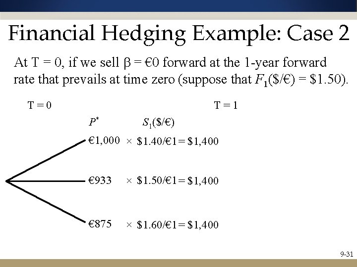
Financial Hedging Example: Case 2 At T = 0, if we sell b = € 0 forward at the 1 -year forward rate that prevails at time zero (suppose that F 1($/€) = $1. 50). T=0 T=1 P* S 1($/€) € 1, 000 × $1. 40/€ 1 = $1, 400 € 933 × $1. 50/€ 1 = $1, 400 € 875 × $1. 60/€ 1 = $1, 400 9 -31

Financial Hedging Example: Case 3 § Financial hedging requires a knowledge of the extent to which the firm’s operating cash flows are affected by the exchange rate. § In an earlier example from Chapter 8, we showed how to hedge case three: simply sell b = € 1, 000 forward or use a money market hedge. State Probability P* S S×P* 1 1/3 € 1, 000 $1. 40/€ $1, 400 2 1/3 € 1, 000 $1. 50/€ $1, 500 3 1/3 € 1, 000 $1. 60/€ $1, 600 Case 3 9 -32

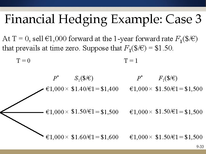
Financial Hedging Example: Case 3 At T = 0, sell € 1, 000 forward at the 1 -year forward rate F 1($/€) that prevails at time zero. Suppose that F 1($/€) = $1. 50. T=0 T=1 P* S 1($/€) P* F 1($/€) € 1, 000 × $1. 40/€ 1 = $1, 400 € 1, 000 × $1. 50/€ 1 = $1, 500 € 1, 000 × $1. 60/€ 1 = $1, 600 € 1, 000 × $1. 50/€ 1 = $1, 500 9 -33