Economic Exposure Sections Measuring economic exposure Managing net

Economic Exposure

Sections Measuring economic exposure Managing (net) asset exposure Operating exposure Managing operating exposure

Economic exposure Changes in exchange rates can affect not only firms that are directly engaged in international trade but also purely domestic firms. If the domestic firm’s products compete with imported goods, then their competitive position is affected by the strength or weakness of the local currency.

Market efficiency Any anticipated changes in the exchange rates would already have been discounted and reflected in the firm’s value. Economic exposure can be defined as the extent to which the value of the firm would be affected by unanticipated changes in exchange rates.

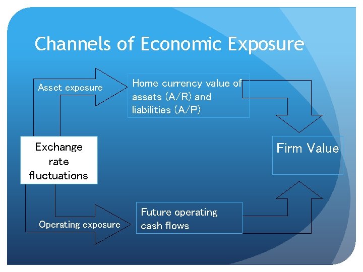
Channels of Economic Exposure Asset exposure Home currency value of assets (A/R) and liabilities (A/P) Exchange rate fluctuations Operating exposure Firm Value Future operating cash flows

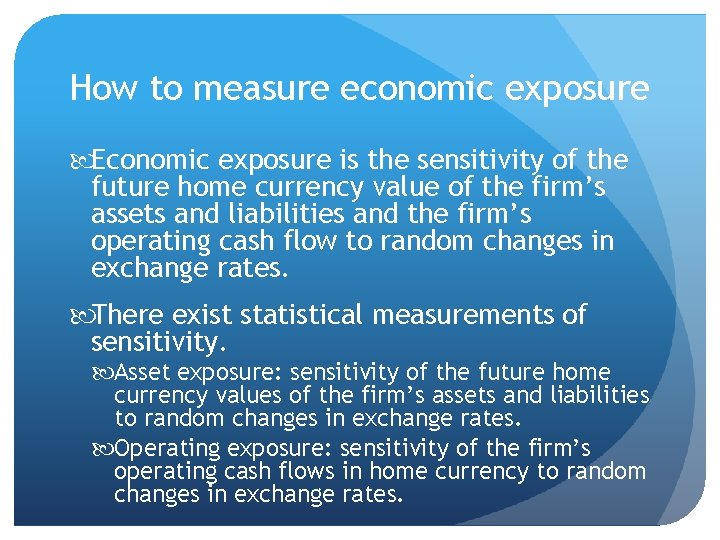
How to measure economic exposure Economic exposure is the sensitivity of the future home currency value of the firm’s assets and liabilities and the firm’s operating cash flow to random changes in exchange rates. There exist statistical measurements of sensitivity. Asset exposure: sensitivity of the future home currency values of the firm’s assets and liabilities to random changes in exchange rates. Operating exposure: sensitivity of the firm’s operating cash flows in home currency to random changes in exchange rates.

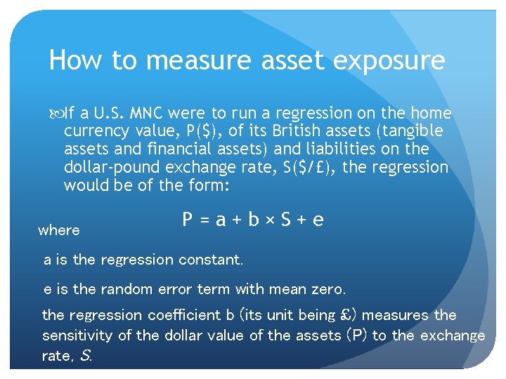
How to measure asset exposure If a U. S. MNC were to run a regression on the home currency value, P($), of its British assets (tangible assets and financial assets) and liabilities on the dollar-pound exchange rate, S($/£), the regression would be of the form: where P=a+b×S+e a is the regression constant. e is the random error term with mean zero. the regression coefficient b (its unit being £) measures the sensitivity of the dollar value of the assets (P) to the exchange rate, S.

Mindful about quotation and units! For the US MNC example: P ($) = a + b (£) × S ($/£) + e. In contrast, if we have a British firm that has an American asset, the quotation and units will change accordingly: P (£) = a + b ($) × S (£/$) + e.

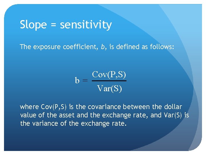
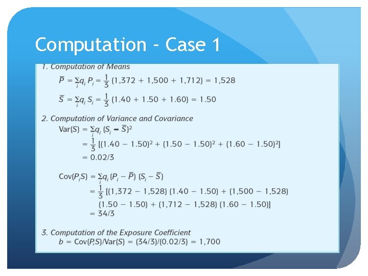
Slope = sensitivity The exposure coefficient, b, is defined as follows: b= Cov(P, S) Var(S) where Cov(P, S) is the covariance between the dollar value of the asset and the exchange rate, and Var(S) is the variance of the exchange rate.

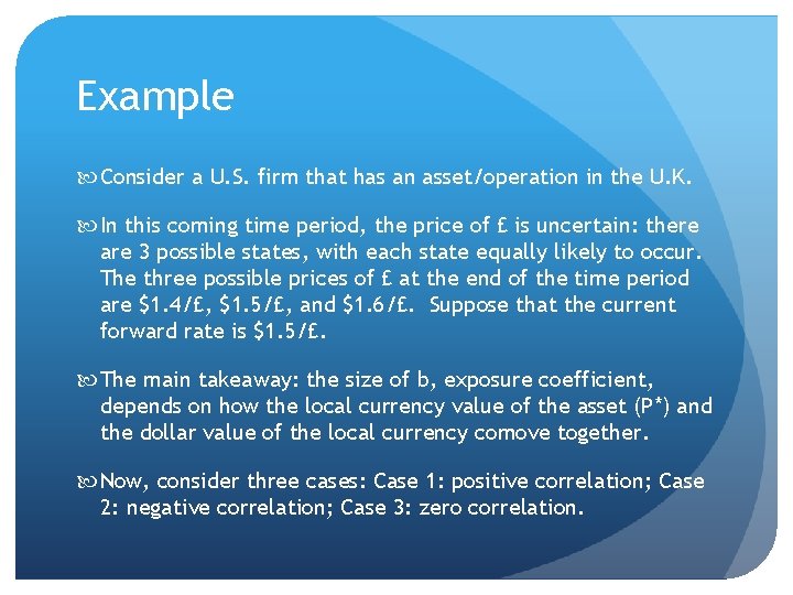
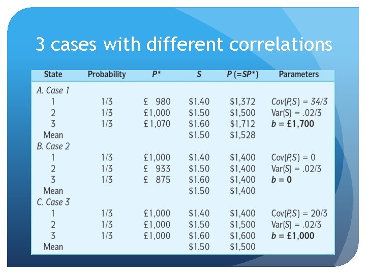
Example Consider a U. S. firm that has an asset/operation in the U. K. In this coming time period, the price of £ is uncertain: there are 3 possible states, with each state equally likely to occur. The three possible prices of £ at the end of the time period are $1. 4/£, $1. 5/£, and $1. 6/£. Suppose that the current forward rate is $1. 5/£. The main takeaway: the size of b, exposure coefficient, depends on how the local currency value of the asset (P*) and the dollar value of the local currency comove together. Now, consider three cases: Case 1: positive correlation; Case 2: negative correlation; Case 3: zero correlation.

3 cases with different correlations

Positive correlation In real life, we would expect a somewhat positive correlation between local currency price of the asset (P*) and the dollar price of local currency (S). That is, Case 1 is a more typical situation in real life. Logic: when hot money flows into a country for whatever reason, it drives up both the dollar price of its currency and the local currency price of its assets. So now let us take a look at the computation for Case 1.

Computation – Case 1 _

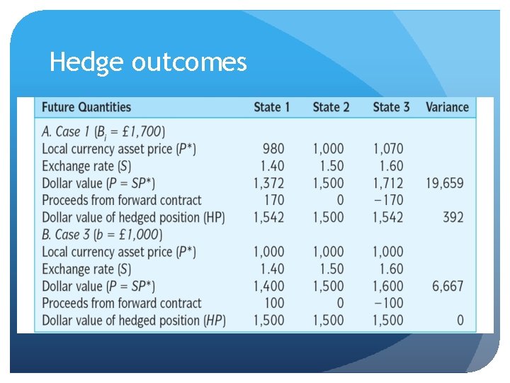
Managing asset exposure When you believe that there is positive correlation between P* and S (i. e. , Case 1), the estimate of the exposure is £ 1, 700. Note that £ 1, 700 is a larger exposure than three possible local currency asset values (£ 980, £ 1, 000, £ 1, 070 ) would suggest. One can use financial contracts to hedge the exposure. For example, the firm can sell £ 1, 700 forward.

Hedge outcomes

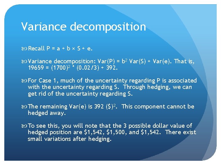
Variance decomposition Recall P = a + b × S + e. Variance decomposition: Var(P) = b 2 Var(S) + Var(e). That is, 19659 = (1700)2 * (0. 02/3) + 392. For Case 1, much of the uncertainty regarding P is associated with the uncertainty regarding S. Through hedging, we can get rid of the uncertainty regarding S. The remaining Var(e) is 392 ($)2. This component cannot be hedged away. To see this, you will note that the 3 possible dollar value of hedged position are $1, 542, $1, 500, and $1, 542. There exist small variations after hedging.

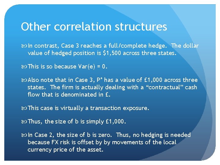
Other correlation structures In contrast, Case 3 reaches a full/complete hedge. The dollar value of hedged position is $1, 500 across three states. This is so because Var(e) = 0. Also note that in Case 3, P* has a value of £ 1, 000 across three states. The firm is actually dealing with a “contractual” cash flow that is denominated in £. This case is virtually a transaction exposure. Thus, the size of b is simply £ 1, 000. In Case 2, the size of b is zero. Thus, no hedging is needed because FX risk is offset by by movements of the local currency price of the asset.

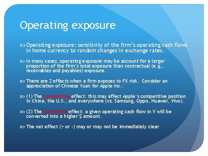
Operating exposure Operating exposure: sensitivity of the firm’s operating cash flows in home currency to random changes in exchange rates. In many cases, operating exposure may be account for a larger proportion of the firm’s total exposure than contractual (e. g. , receivables and payables) exposure. There are 2 effects when a firm exposes to FX risk. Consider an appreciation of Chinese Yuan for Apple Inc. : (1) The competitive effect: this may affect Apple’s competitive position in China, the U. S. , and everywhere (vs. Samsung, Oppo, Huawei, Vivo). (2) The conversion effect: a given operating cash flow in ¥ will be converted into a higher $ amount. The net effect (+ or -) may or may not be immediately clear.

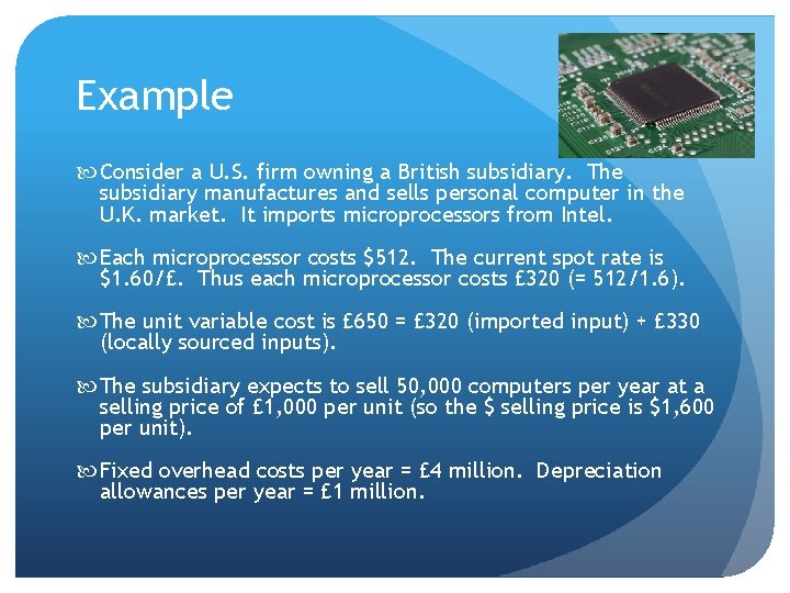
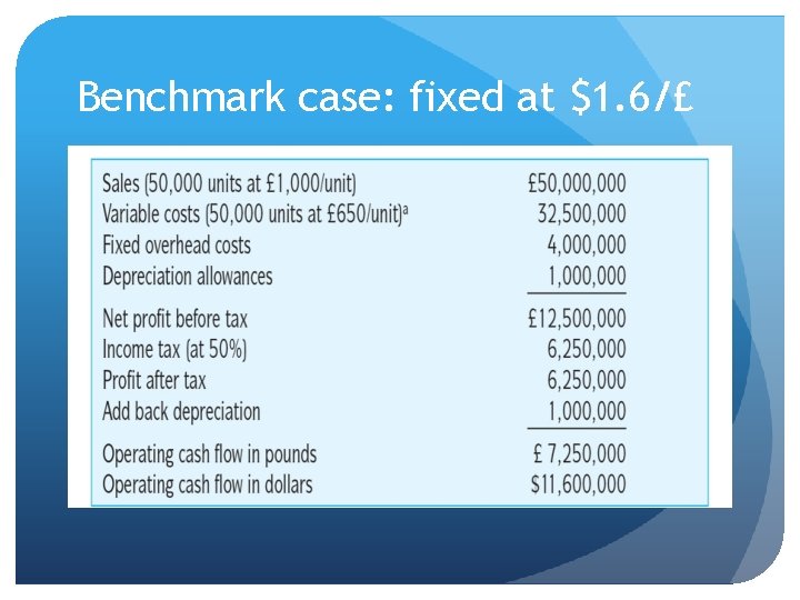
Example Consider a U. S. firm owning a British subsidiary. The subsidiary manufactures and sells personal computer in the U. K. market. It imports microprocessors from Intel. Each microprocessor costs $512. The current spot rate is $1. 60/£. Thus each microprocessor costs £ 320 (= 512/1. 6). The unit variable cost is £ 650 = £ 320 (imported input) + £ 330 (locally sourced inputs). The subsidiary expects to sell 50, 000 computers per year at a selling price of £ 1, 000 per unit (so the $ selling price is $1, 600 per unit). Fixed overhead costs per year = £ 4 million. Depreciation allowances per year = £ 1 million.

Benchmark case: fixed at $1. 6/£

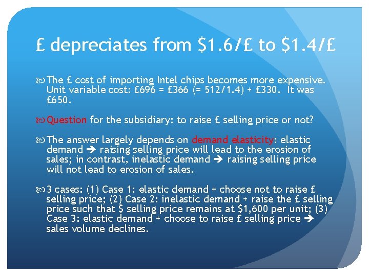
£ depreciates from $1. 6/£ to $1. 4/£ The £ cost of importing Intel chips becomes more expensive. Unit variable cost: £ 696 = £ 366 (= 512/1. 4) + £ 330. It was £ 650. Question for the subsidiary: to raise £ selling price or not? The answer largely depends on demand elasticity: elastic demand raising selling price will lead to the erosion of sales; in contrast, inelastic demand raising selling price will not lead to erosion of sales. 3 cases: (1) Case 1: elastic demand + choose not to raise £ selling price; (2) Case 2: inelastic demand + raise the £ selling price such that $ selling price remains at $1, 600 per unit; (3) Case 3: elastic demand + choose to raise £ selling price sales volume declines.

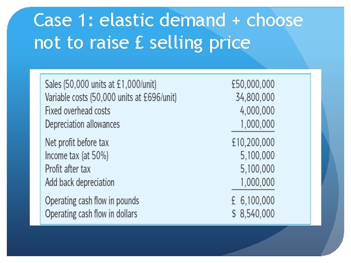
Case 1: elastic demand + choose not to raise £ selling price

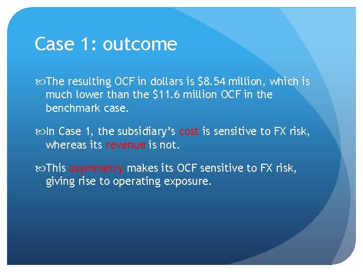
Case 1: outcome The resulting OCF in dollars is $8. 54 million, which is much lower than the $11. 6 million OCF in the benchmark case. In Case 1, the subsidiary’s cost is sensitive to FX risk, whereas its revenue is not. This asymmetry makes its OCF sensitive to FX risk, giving rise to operating exposure.

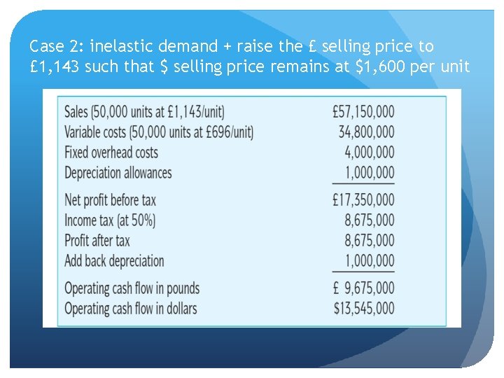
Case 2: inelastic demand + raise the £ selling price to £ 1, 143 such that $ selling price remains at $1, 600 per unit

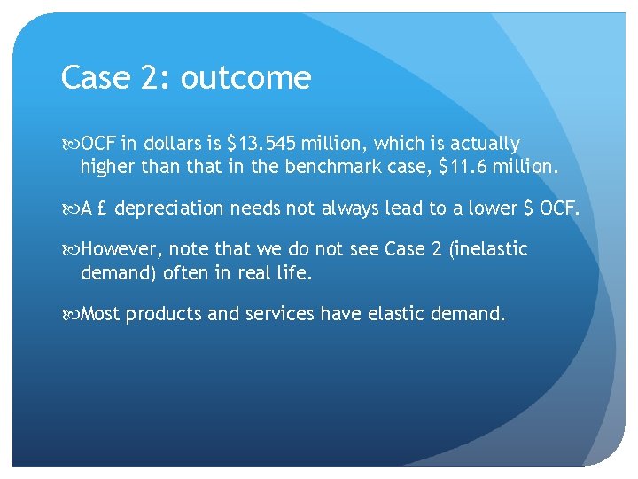
Case 2: outcome OCF in dollars is $13. 545 million, which is actually higher than that in the benchmark case, $11. 6 million. A £ depreciation needs not always lead to a lower $ OCF. However, note that we do not see Case 2 (inelastic demand) often in real life. Most products and services have elastic demand.

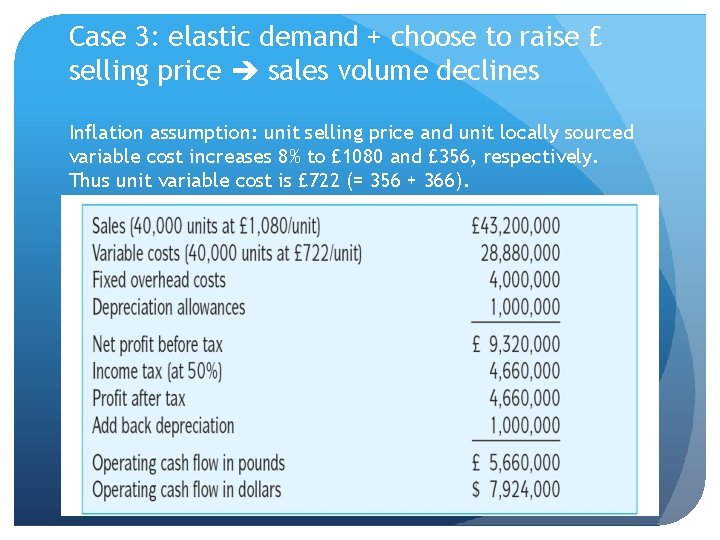
Case 3: elastic demand + choose to raise £ selling price sales volume declines Inflation assumption: unit selling price and unit locally sourced variable cost increases 8% to £ 1080 and £ 356, respectively. Thus unit variable cost is £ 722 (= 356 + 366).

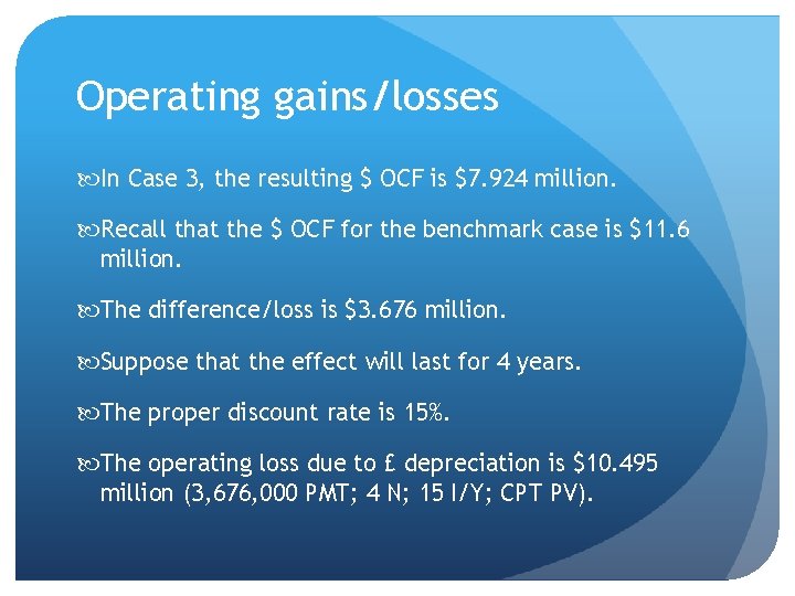
Operating gains/losses In Case 3, the resulting $ OCF is $7. 924 million. Recall that the $ OCF for the benchmark case is $11. 6 million. The difference/loss is $3. 676 million. Suppose that the effect will last for 4 years. The proper discount rate is 15%. The operating loss due to £ depreciation is $10. 495 million (3, 676, 000 PMT; 4 N; 15 I/Y; CPT PV).

Determinants of operating exposure The above example demonstrated that operating exposure cannot be readily determined from the firm’s accounting statements as can transaction exposure. The firm’s operating exposure is determined by: The market structure of inputs and products; how competitive or how monopolistic the markets facing the firm are. The firm’s ability to adjust its markets, product mix, and sourcing in response to exchange rate changes.

Managing operating exposure A firm is exposed to exchange rate risk mainly through the effect of FX changes in its competitive position. Thus, operation exposure management needs to be a part of the firm’s long-term strategic planning.

Managing strategies Selecting low cost production sites Flexible sourcing policy Diversification of the market R&D and product differentiation Financial hedging

Selecting (low cost) production sites A firm may wish to diversify the location of its production sites to mitigate the effect of exchange rate movements. For example, Honda built North American factories in response to a strong yen, but later found itself importing more cars from Japan due to a weak yen. E. g. , Mexico, China, Vietnam. Downside: economies of scale.

Flexible sourcing policy Sourcing does not apply only to components, but also to “guest workers. ” For example, Japan Air Lines hired foreign crews to remain competitive in international routes in the face of a strong yen, but later contemplated a reverse strategy in the face of a weak yen and rising domestic unemployment.

Diversification of the market Selling in multiple markets to take advantage of economies of scale and diversification of exchange rate risk.

R&D and product differentiation Successful research and development (R&D) allows for: Cost-cutting Enhanced productivity Product differentiation Successful product differentiation gives the firm less elastic demand—which may translate into less exchange rate risk.

Financial hedging Firms expose to FX risk mainly through the effect of FX variability on its competitive position. Thus, managing operating exposure is strategic in nature. In contrast, financial hedging is more about stabilize the firm’s cash flows in the near term. Financial hedging involves the use of derivative securities such as currency swaps, futures, forwards, and currency options.

End-of-chapter Questions: 1 -9, 11. Problems: 1 -3.