Management of Economic Chapter Nine Exposure Copyright 2018

Management of Economic Chapter Nine Exposure Copyright © 2018 by the Mc. Graw-Hill Companies, Inc. All rights reserved.

Chapter Outline • • • How to Measure Economic Exposure Operating Exposure: Definition An Illustration of Operating Exposure Determinants of Operating Exposure Managing Operating Exposure Summary Copyright © 2018 by the Mc. Graw-Hill Companies, Inc. All rights reserved. 9 -2

Economic Exposure • Changes in exchange rates can affect not only firms that are directly engaged in international trade but also purely domestic firms. • If the domestic firm’s products compete with imported goods, then their competitive position is affected by the strength or weakness of the local currency. Copyright © 2018 by the Mc. Graw-Hill Companies, Inc. All rights reserved. 9 -3

Economic Exposure • Consider a U. S. bicycle manufacturer who sources, produces, and sells only in the U. S. • Since the firm’s product competes against imported bicycles, it is subject to foreign exchange exposure. • Their customers are comparing the cost and features of the domestic bicycle against Japanese, British, and Italian bicycles. Copyright © 2018 by the Mc. Graw-Hill Companies, Inc. All rights reserved. 9 -4

Economic Exposure • Exchange rate risk is applied to the firm’s competitive position. • Any anticipated changes in the exchange rates would already have been discounted and reflected in the firm’s value. • Economic exposure can be defined as the extent to which the value of the firm would be affected by unanticipated changes in exchange rates. Copyright © 2018 by the Mc. Graw-Hill Companies, Inc. All rights reserved. 9 -5

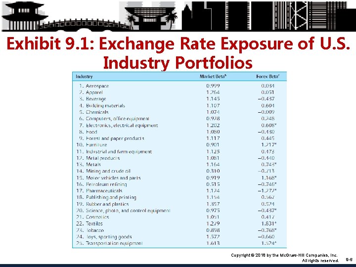
Exhibit 9. 1: Exchange Rate Exposure of U. S. Industry Portfolios Copyright © 2018 by the Mc. Graw-Hill Companies, Inc. All rights reserved. 9 -6

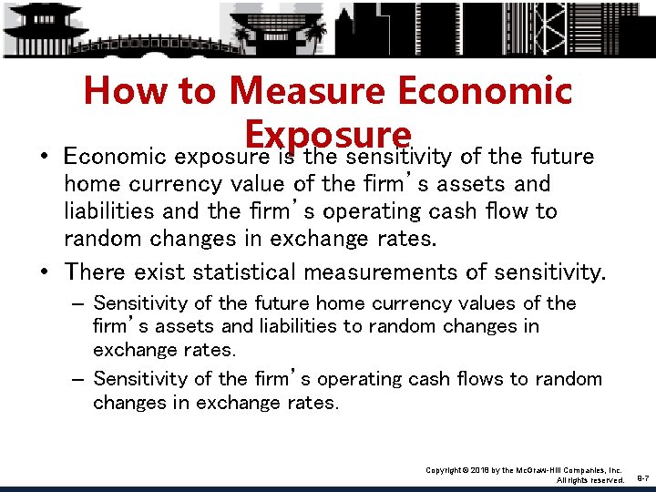
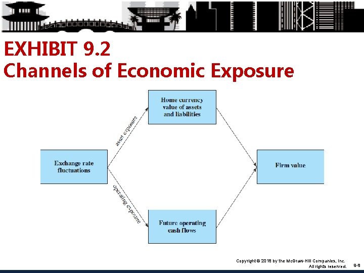
• How to Measure Economic Exposure Economic exposure is the sensitivity of the future home currency value of the firm’s assets and liabilities and the firm’s operating cash flow to random changes in exchange rates. • There exist statistical measurements of sensitivity. – Sensitivity of the future home currency values of the firm’s assets and liabilities to random changes in exchange rates. – Sensitivity of the firm’s operating cash flows to random changes in exchange rates. Copyright © 2018 by the Mc. Graw-Hill Companies, Inc. All rights reserved. 9 -7

EXHIBIT 9. 2 Channels of Economic Exposure Copyright © 2018 by the Mc. Graw-Hill Companies, Inc. All rights reserved. 9 -8

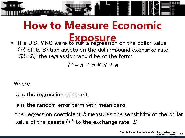
• How to Measure Economic Exposure If a U. S. MNC were to run a regression on the dollar value (P) of its British assets on the dollar-pound exchange rate, S($/£), the regression would be of the form: P = a + b×S + e Where a is the regression constant. e is the random error term with mean zero. the regression coefficient b measures the sensitivity of the dollar value of the assets (P) to the exchange rate, S. Copyright © 2018 by the Mc. Graw-Hill Companies, Inc. All rights reserved. 9 -9

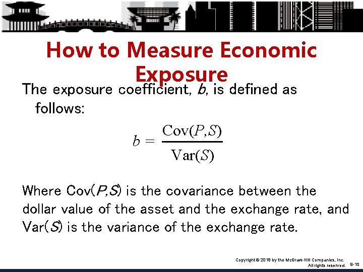
How to Measure Economic Exposure The exposure coefficient, b, is defined as follows: Cov(P, S) b= Var(S) Where Cov(P, S) is the covariance between the dollar value of the asset and the exchange rate, and Var(S) is the variance of the exchange rate. Copyright © 2018 by the Mc. Graw-Hill Companies, Inc. All rights reserved. 9 -10

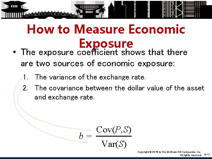
How to Measure Economic Exposure • The exposure coefficient shows that there are two sources of economic exposure: 1. The variance of the exchange rate. 2. The covariance between the dollar value of the asset and exchange rate. b= Cov(P, S) Var(S) Copyright © 2018 by the Mc. Graw-Hill Companies, Inc. All rights reserved. 9 -11

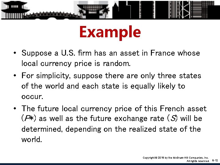
Example • Suppose a U. S. firm has an asset in France whose local currency price is random. • For simplicity, suppose there are only three states of the world and each state is equally likely to occur. • The future local currency price of this French asset (P*) as well as the future exchange rate (S) will be determined, depending on the realized state of the world. Copyright © 2018 by the Mc. Graw-Hill Companies, Inc. All rights reserved. 9 -12

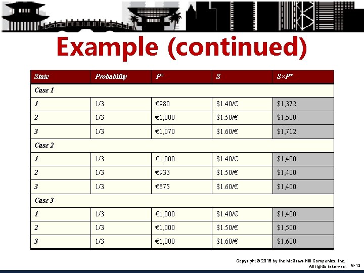
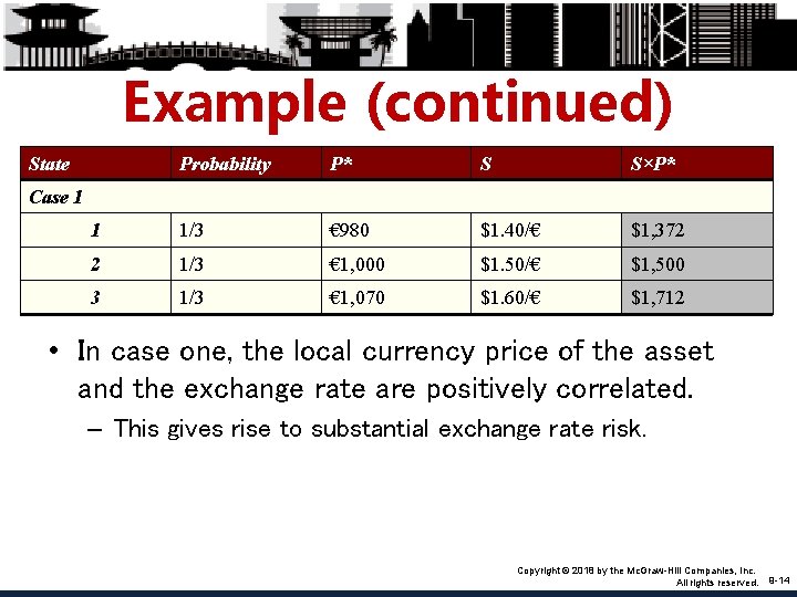
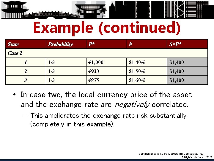
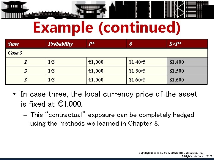
Example (continued) State Probability P* S S×P* 1 1/3 € 980 $1. 40/€ $1, 372 2 1/3 € 1, 000 $1. 50/€ $1, 500 3 1/3 € 1, 070 $1. 60/€ $1, 712 1 1/3 € 1, 000 $1. 40/€ $1, 400 2 1/3 € 933 $1. 50/€ $1, 400 3 1/3 € 875 $1. 60/€ $1, 400 1 1/3 € 1, 000 $1. 40/€ $1, 400 2 1/3 € 1, 000 $1. 50/€ $1, 500 3 1/3 € 1, 000 $1. 60/€ $1, 600 Case 1 Case 2 Case 3 Copyright © 2018 by the Mc. Graw-Hill Companies, Inc. All rights reserved. 9 -13

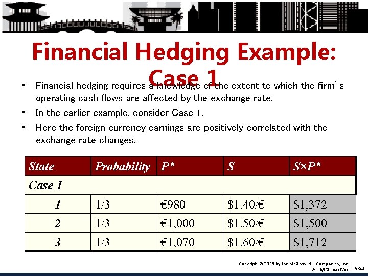
Example (continued) State Probability P* S S×P* 1 1/3 € 980 $1. 40/€ $1, 372 2 1/3 € 1, 000 $1. 50/€ $1, 500 3 1/3 € 1, 070 $1. 60/€ $1, 712 Case 1 • In case one, the local currency price of the asset and the exchange rate are positively correlated. – This gives rise to substantial exchange rate risk. Copyright © 2018 by the Mc. Graw-Hill Companies, Inc. All rights reserved. 9 -14

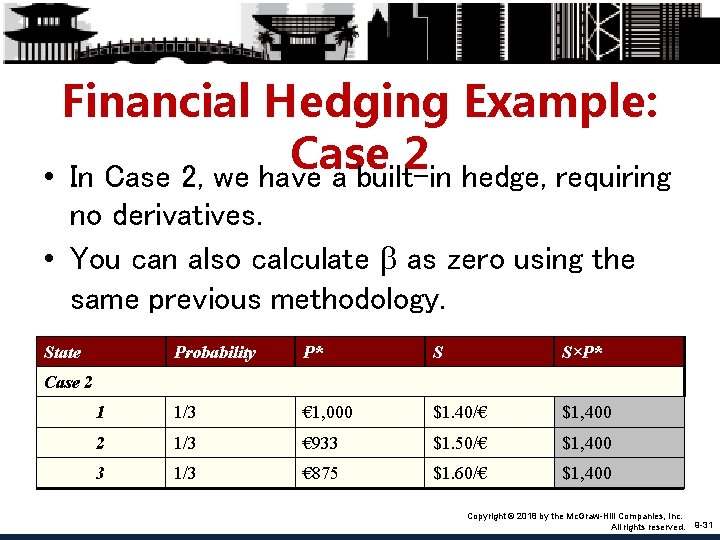
Example (continued) State Probability P* S S×P* 1 1/3 € 1, 000 $1. 40/€ $1, 400 2 1/3 € 933 $1. 50/€ $1, 400 3 1/3 € 875 $1. 60/€ $1, 400 Case 2 • In case two, the local currency price of the asset and the exchange rate are negatively correlated. – This ameliorates the exchange rate risk substantially (completely in this example). Copyright © 2018 by the Mc. Graw-Hill Companies, Inc. All rights reserved. 9 -15

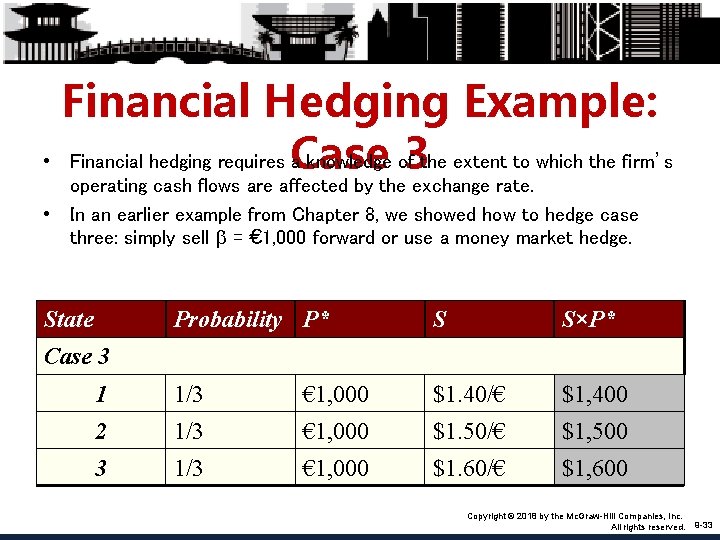
Example (continued) State Probability P* S S×P* 1 1/3 € 1, 000 $1. 40/€ $1, 400 2 1/3 € 1, 000 $1. 50/€ $1, 500 3 1/3 € 1, 000 $1. 60/€ $1, 600 Case 3 • In case three, the local currency price of the asset is fixed at € 1, 000. – This “contractual” exposure can be completely hedged using the methods we learned in Chapter 8. Copyright © 2018 by the Mc. Graw-Hill Companies, Inc. All rights reserved. 9 -16

• Operating Exposure: The effect of. Definition random changes in exchange rates on the firm’s competitive position, which is not readily measurable. • A good definition of operating exposure is the extent to which the firm’s operating cash flows are affected by the exchange rate. Copyright © 2018 by the Mc. Graw-Hill Companies, Inc. All rights reserved. 9 -17

An Illustration of Operating Exposure • There was an enormous shortage in the shipping market from Asia due to the Asian currency crisis. • This affected not only the shipping companies, who enjoyed “boom times, ” but also retailers, who experienced increased costs and delays. Copyright © 2018 by the Mc. Graw-Hill Companies, Inc. All rights reserved. 9 -18

An Illustration of Operating Exposure • Note that the exposure for the retailers has two components. – The competitive effect: • Difficulties and increased costs of shipping – The conversion effect: • Lower dollar prices of imports due to foreign currency exchange rate depreciation. Copyright © 2018 by the Mc. Graw-Hill Companies, Inc. All rights reserved. 9 -19

• • Determinants of Operating Exposure Recall that operating exposure cannot be readily determined from the firm’s accounting statements as can transaction exposure. The firm’s operating exposure is determined by: – The market structure of inputs and products; how competitive or how monopolistic the markets facing the firm are. – The firm’s ability to adjust its markets, product mix, and sourcing in response to exchange rate changes. Copyright © 2018 by the Mc. Graw-Hill Companies, Inc. All rights reserved. 9 -20

• • • Managing Operating Selecting Low. Exposure Cost Production Sites Flexible Sourcing Policy Diversification of the Market R&D and Product Differentiation Financial Hedging Copyright © 2018 by the Mc. Graw-Hill Companies, Inc. All rights reserved. 9 -21

• Selecting Low Cost Production Sites A firm may wish to diversify the location of its production sites to mitigate the effect of exchange rate movements. • For example, Honda built North American factories in response to a strong yen, but later found itself importing more cars from Japan due to a weak yen and increased exchange rate volatility. Copyright © 2018 by the Mc. Graw-Hill Companies, Inc. All rights reserved. 9 -22

Flexible Sourcing Policy • Sourcing does not apply only to components, but also to “guest workers. ” • For example, Japan Air Lines hired foreign crews to remain competitive in international routes in the face of a strong yen, but later contemplated a reverse strategy in the face of a weak yen and rising domestic unemployment. Copyright © 2018 by the Mc. Graw-Hill Companies, Inc. All rights reserved. 9 -23

• Diversification of the Market Selling in multiple markets to take advantage of economies of scale and diversification of exchange rate risk. Copyright © 2018 by the Mc. Graw-Hill Companies, Inc. All rights reserved. 9 -24

• R&D and Product Differentiation Successful research and development (R&D) allows for: – Cost-cutting – Enhanced productivity – Product differentiation • Successful product differentiation gives the firm less elastic demand—which may translate into less exchange rate risk. Copyright © 2018 by the Mc. Graw-Hill Companies, Inc. All rights reserved. 9 -25

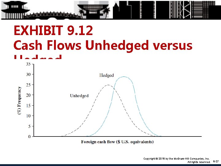
Financial Hedging • The goal is to stabilize the firm’s cash flows in the near term. • Financial hedging is distinct from operational hedging. • Financial hedging involves the use of derivative securities such as currency swaps, futures, forwards, and currency options, among others. Copyright © 2018 by the Mc. Graw-Hill Companies, Inc. All rights reserved. 9 -26

EXHIBIT 9. 12 Cash Flows Unhedged versus Hedged Copyright © 2018 by the Mc. Graw-Hill Companies, Inc. All rights reserved. 9 -27

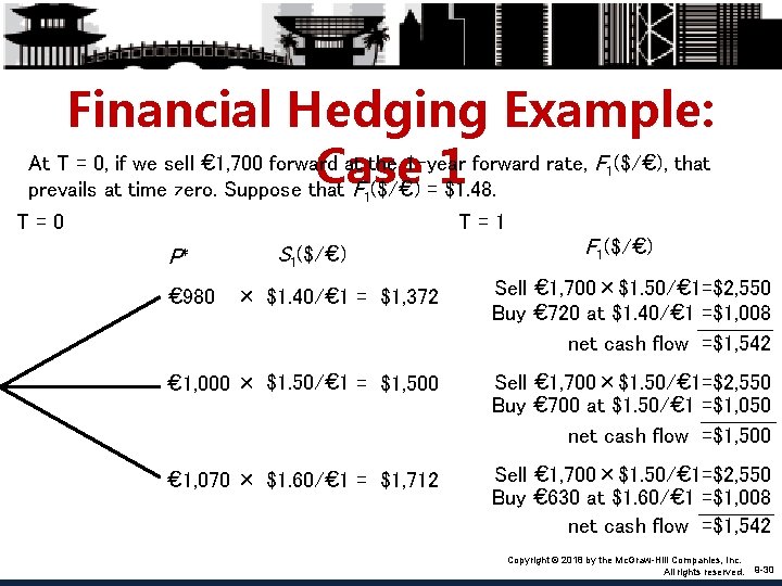
Financial Hedging Example: 1 the extent to which the firm’s • Financial hedging requires Case a knowledge of operating cash flows are affected by the exchange rate. • In the earlier example, consider Case 1. • Here the foreign currency earnings are positively correlated with the exchange rate changes. State Probability P* S S×P* 1 1/3 € 980 $1. 40/€ $1, 372 2 1/3 € 1, 000 $1. 50/€ $1, 500 3 1/3 € 1, 070 $1. 60/€ $1, 712 Case 1 Copyright © 2018 by the Mc. Graw-Hill Companies, Inc. All rights reserved. 9 -28

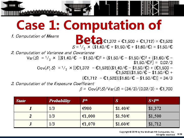
Case 1: Computation of Beta 1. Computation of Means P = 1/3 × (€ 1, 372 + € 1, 500 + € 1, 712) = € 1, 528 S = 1/3 × ($1. 40/€ + $1. 50/€ + $1. 60/€) = $1. 50/€ 2. Computation of Variance and Covariance Var(S) = 1/3 × [($1. 40/€ – $1. 50/€)2 + ($1. 50/€ – $1. 50/€)2 + ($1. 60/€ – $1. 50/€)2] = 0. 02/3 Cov(Pi S) = 1/3 ×[(€ 1, 372 – € 1, 528)($1. 40/€ – $1. 50/€) + (€ 1, 500 – € 1, 528)($1. 50/€ – $1. 50/€) + (€ 1, 712 – € 1, 528)($1. 60/€ – $1. 50/€)] = 34/3 3. Computation of the Exposure Coefficient b = Cov(P, S)/Var(S) = (34/3)/(0. 02/3) = € 1, 700 State Probability P* S S×P* 1 1/3 € 980 $1. 40/€ $1, 372 2 1/3 € 1, 000 $1. 50/€ $1, 500 3 1/3 € 1, 070 $1. 60/€ $1, 712 Copyright © 2018 by the Mc. Graw-Hill Companies, Inc. All rights reserved. 9 -29

Financial Hedging Example: At T = 0, if we sell € 1, 700 forward at the 1 -year forward rate, F ($/€), that Case 1 prevails at time zero. Suppose that F ($/€) = $1. 48. 1 1 T=0 T=1 P* S 1($/€) F 1($/€) € 980 × $1. 40/€ 1 = $1, 372 Sell € 1, 700×$1. 50/€ 1=$2, 550 Buy € 720 at $1. 40/€ 1 =$1, 008 net cash flow =$1, 542 € 1, 000 × $1. 50/€ 1 = $1, 500 Sell € 1, 700×$1. 50/€ 1=$2, 550 Buy € 700 at $1. 50/€ 1 =$1, 050 net cash flow =$1, 500 € 1, 070 × $1. 60/€ 1 = $1, 712 Sell € 1, 700×$1. 50/€ 1=$2, 550 Buy € 630 at $1. 60/€ 1 =$1, 008 net cash flow =$1, 542 Copyright © 2018 by the Mc. Graw-Hill Companies, Inc. All rights reserved. 9 -30

Financial Hedging Example: Case 2 • In Case 2, we have a built-in hedge, requiring no derivatives. • You can also calculate b as zero using the same previous methodology. State Probability P* S S×P* 1 1/3 € 1, 000 $1. 40/€ $1, 400 2 1/3 € 933 $1. 50/€ $1, 400 3 1/3 € 875 $1. 60/€ $1, 400 Case 2 Copyright © 2018 by the Mc. Graw-Hill Companies, Inc. All rights reserved. 9 -31

Financial Hedging Example: At T = 0, if we sell b = € 0 forward at the 1 -year forward rate that prevails at Case 2 time zero (suppose that F ($/€) = $1. 50). 1 T=0 T=1 P* S 1($/€) € 1, 000 × $1. 40/€ 1 = $1, 400 € 933 × $1. 50/€ 1 = $1, 400 € 875 × $1. 60/€ 1 = $1, 400 Copyright © 2018 by the Mc. Graw-Hill Companies, Inc. All rights reserved. 9 -32

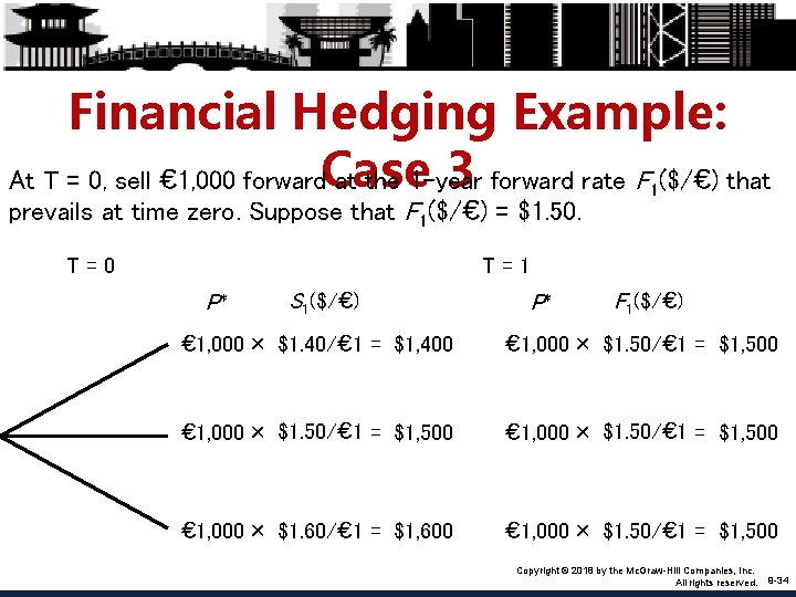
Financial Hedging Example: • Financial hedging requires Case a knowledge of 3 the extent to which the firm’s operating cash flows are affected by the exchange rate. • In an earlier example from Chapter 8, we showed how to hedge case three: simply sell b = € 1, 000 forward or use a money market hedge. State Probability P* S S×P* 1 1/3 € 1, 000 $1. 40/€ $1, 400 2 1/3 € 1, 000 $1. 50/€ $1, 500 3 1/3 € 1, 000 $1. 60/€ $1, 600 Case 3 Copyright © 2018 by the Mc. Graw-Hill Companies, Inc. All rights reserved. 9 -33

Financial Hedging Example: 3 forward rate F ($/€) that At T = 0, sell € 1, 000 forward. Case at the 1 -year prevails at time zero. Suppose that F 1($/€) = $1. 50. T=0 1 T=1 P* S 1($/€) P* F 1($/€) € 1, 000 × $1. 40/€ 1 = $1, 400 € 1, 000 × $1. 50/€ 1 = $1, 500 € 1, 000 × $1. 60/€ 1 = $1, 600 € 1, 000 × $1. 50/€ 1 = $1, 500 Copyright © 2018 by the Mc. Graw-Hill Companies, Inc. All rights reserved. 9 -34

Summary • Exchange rate changes can systematically affect the value of the firm by influencing the firm’s operating cash flows as well as the domestic currency values of its assets and liabilities. • It is conventional to classify foreign currency exposure into three classes: – Economic exposure can be defined as the extent to which the value of the firm would be affected by unexpected changes in exchange rates. – Transaction exposure is defined as the sensitivity of realized domestic currency values of the firm’s contractual cash flows denominated in foreign currencies to unexpected exchange rate changes. – Translation exposure refers to the potential that the firm’s consolidated financial statements can be affected by changes in exchange rates. Copyright © 2018 by the Mc. Graw-Hill Companies, Inc. All rights reserved. 9 -35

Summary (continued) • If the firm has an asset in a foreign country, its exposure to currency risk can be properly measured by the coefficient in regressing the dollar value of the foreign asset on the exchange rate. – Once the magnitude of exposure is known, the firm can hedge the exposure simply by selling the exposure forward. • Unlike the exposure of assets and liabilities that are listed in accounting statements, operating exposure depends on the effect of random exchange rate changes on the firm’s future cash flows, which are not readily measurable. Despite this difficulty, it is important to properly manage operating exposure since operating exposure may account for a larger portion of the firm’s total exposure than contractual exposure. Copyright © 2018 by the Mc. Graw-Hill Companies, Inc. All rights reserved. 9 -36

Summary (concluding) • A firm’s operating exposure is determined by – (a) the structure of the markets in which the firm sources its inputs and sells its products, and – (b) the firm’s ability to mitigate the effect of exchange rate changes on its competitive position by adjusting markets, product mix, and sourcing. • Since a firm is exposed to exchange risk mainly via the effect of exchange rate changes on its competitive position, it is important to consider exchange exposure management in the context of the firm’s overall long-term strategic plan. The objective of exposure management is to stabilize cash flow in the face of fluctuating exchange rates. Copyright © 2018 by the Mc. Graw-Hill Companies, Inc. All rights reserved. 9 -37

Summary (concluded) • To manage operating exposure, the firm can use various strategies, such as – – – (a) choosing low-cost production sites, (b) maintaining flexible sourcing policy, (c) diversification of the market, (d) product differentiation, and (e) financial hedging using currency options and forward contracts. Copyright © 2018 by the Mc. Graw-Hill Companies, Inc. All rights reserved. 9 -38