Making Decisions Against an Opponent An application of

Making Decisions Against an Opponent: An application of Mathematical Optimization ISYE 2030 Monday, October 2, 2000 Dr. Joel Sokol jsokol@isye. gatech. edu

Making Decisions Against an Opponent • Two people/teams in competition • Outcome depends on both sides’ simultaneous decisions • Many examples in business, sports, economics, and even everyday life

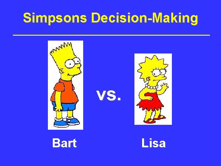
Simpsons Decision-Making vs. Bart Lisa

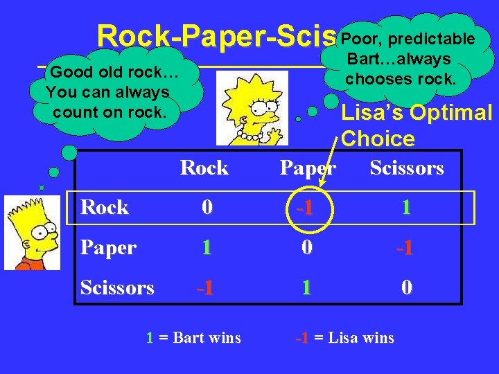
Poor, predictable Rock-Paper-Scissors Bart…always chooses rock. Good old rock… You can always count on rock. Rock Lisa’s Optimal Choice Paper Scissors Rock 0 -1 1 Paper 1 0 -1 Scissors -1 1 0 1 = Bart wins -1 = Lisa wins

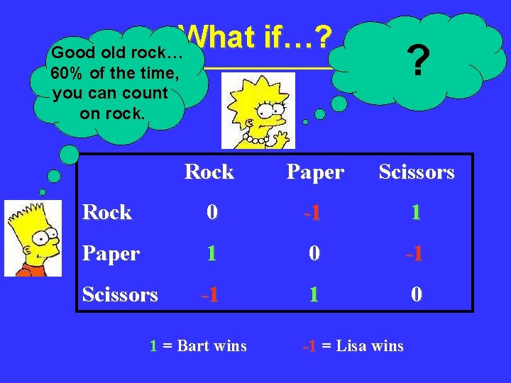
What if…? Good old rock… ? 60% of the time, you can count on rock. Rock Paper Scissors Rock 0 -1 1 Paper 1 0 -1 Scissors -1 1 0 1 = Bart wins -1 = Lisa wins

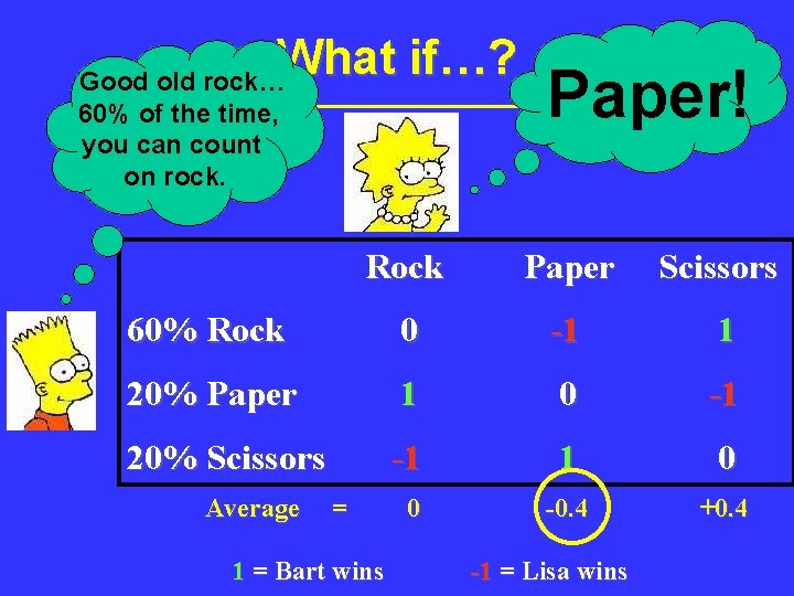
What if…? Good old rock… 60% of the time, you can count on rock. Paper! Rock Paper Scissors 60% Rock 0 -1 1 20% Paper 1 0 -1 20% Scissors -1 1 0 0 -0. 4 +0. 4 Average = 1 = Bart wins -1 = Lisa wins

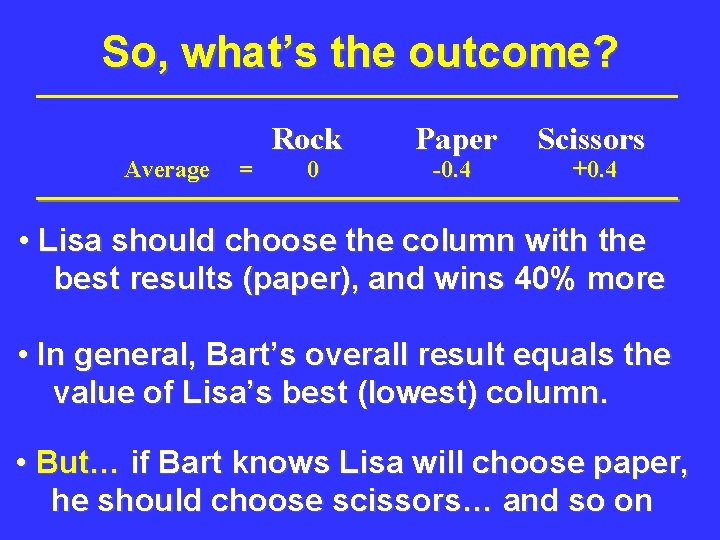
So, what’s the outcome? Average = Rock 0 Paper -0. 4 Scissors +0. 4 • Lisa should choose the column with the best results (paper), and wins 40% more • In general, Bart’s overall result equals the value of Lisa’s best (lowest) column. • But… if Bart knows Lisa will choose paper, he should choose scissors… and so on

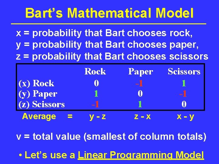
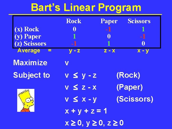
Bart’s Mathematical Model x = probability that Bart chooses rock, y = probability that Bart chooses paper, z = probability that Bart chooses scissors Rock Paper Scissors (x) Rock 0 -1 1 (y) Paper 1 0 -1 (z) Scissors -1 1 0 Average = y-z z-x x-y v = total value (smallest of column totals) • Let’s use a Linear Programming Model

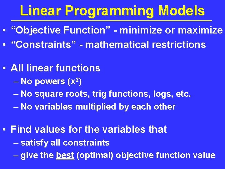
Linear Programming Models • “Objective Function” - minimize or maximize • “Constraints” - mathematical restrictions • All linear functions – No powers (x 2) – No square roots, trig functions, logs, etc. – No variables multiplied by each other • Find values for the variables that – satisfy all constraints – give the best (optimal) objective function value

Bart’s Linear Program (x) Rock (y) Paper (z) Scissors Average = Rock 0 1 -1 y-z Paper -1 0 1 z-x Scissors 1 -1 0 x-y Maximize v Subject to v y-z (Rock) v z-x (Paper) v x-y (Scissors) x+y+z=1 x 0, y 0, z 0

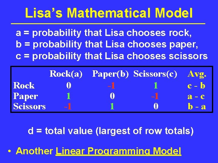
Lisa’s Mathematical Model a = probability that Lisa chooses rock, b = probability that Lisa chooses paper, c = probability that Lisa chooses scissors Rock(a) Paper(b) Scissors(c) Rock 0 -1 1 Paper 1 0 -1 Scissors -1 1 0 Avg. c-b a-c b-a d = total value (largest of row totals) • Another Linear Programming Model

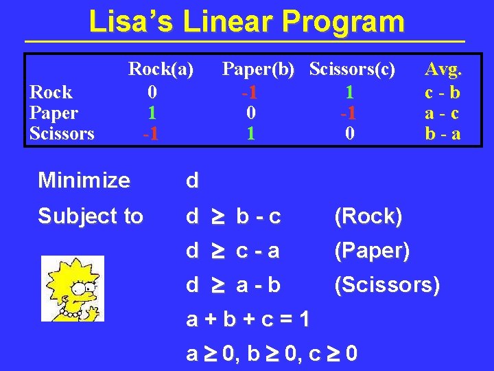
Lisa’s Linear Program Rock Paper Scissors Rock(a) 0 1 -1 Paper(b) Scissors(c) -1 1 0 Avg. c-b a-c b-a Minimize d Subject to d b-c (Rock) d c-a (Paper) d a-b (Scissors) a+b+c=1 a 0, b 0, c 0

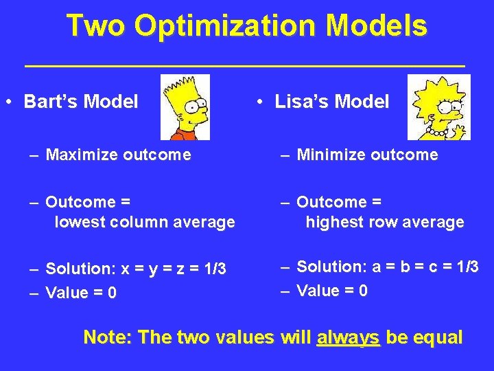
Two Optimization Models • Bart’s Model • Lisa’s Model – Maximize outcome – Minimize outcome – Outcome = lowest column average – Outcome = highest row average – Solution: x = y = z = 1/3 – Value = 0 – Solution: a = b = c = 1/3 – Value = 0 Note: The two values will always be equal

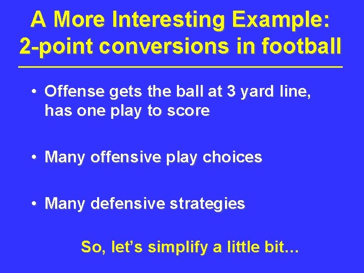
A More Interesting Example: 2 -point conversions in football • Offense gets the ball at 3 yard line, has one play to score • Many offensive play choices • Many defensive strategies So, let’s simplify a little bit…

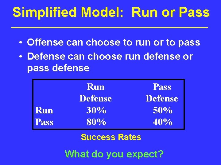
Simplified Model: Run or Pass • Offense can choose to run or to pass • Defense can choose run defense or pass defense Run Pass Run Defense 30% 80% Pass Defense 50% 40% Success Rates What do you expect?

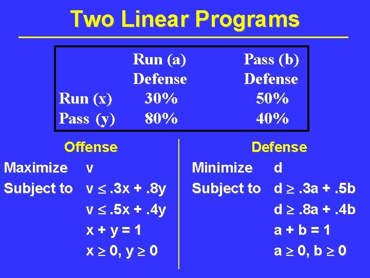
Two Linear Programs Run (x) Pass (y) Run (a) Defense 30% 80% Offense Maximize v Subject to v . 3 x +. 8 y v . 5 x +. 4 y x+y=1 x 0, y 0 Pass (b) Defense 50% 40% Defense Minimize d Subject to d . 3 a +. 5 b d . 8 a +. 4 b a+b=1 a 0, b 0

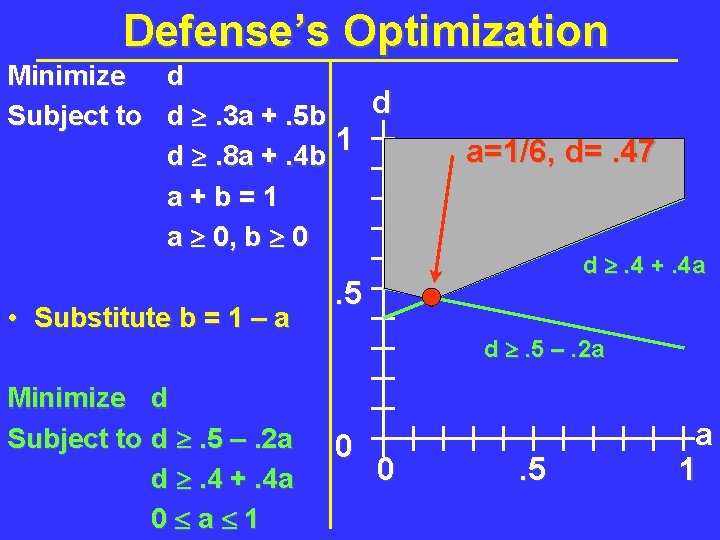
Defense’s Optimization Minimize d d Subject to d . 3 a +. 5 b 1 d . 8 a +. 4 b a+b=1 a 0, b 0 • Substitute b = 1 – a Minimize d Subject to d . 5 –. 2 a d . 4 +. 4 a 0 a 1 a=1/6, d=. 47 d . 4 +. 4 a . 5 d . 5 –. 2 a 0 0 . 5 a 1

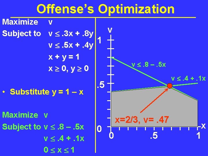
Offense’s Optimization Maximize v v Subject to v . 3 x +. 8 y 1 v . 5 x +. 4 y x+y=1 x 0, y 0 • Substitute y = 1 – x Maximize v Subject to v . 8 –. 5 x v . 4 +. 1 x 0 x 1 v . 8 –. 5 x v . 4 +. 1 x . 5 0 x=2/3, v=. 47 0 . 5 x 1

Summary • Start with a complex problem (making decisions against an opponent) • Create a simplified mathematical model (Optimization/linear programming) • Use the model to suggest a strategy (in this case, a surprising strategy!) Slides at www. isye. gatech. edu/~jsokol/2030. ppt