Machine Learning CSE 6740CS 7641ISYE 6740 Fall 2012

Machine Learning CSE 6740/CS 7641/ISYE 6740, Fall 2012 Tutorial on Basic Probability Le Song Based on Slides from Eric Xing, CMU Reading: Chap. 1&2, CB & Chap 5, 6, TM

What is this? l Classical AI and ML research ignored this phenomena l Another example l you want to catch a flight at 10: 00 am from Pitt to SF, can I make it if I leave at 8 am and take a 28 X at CMU? l partial observability (road state, other drivers' plans, etc. ) l noisy sensors (radio traffic reports) l uncertainty in action outcomes (flat tire, etc. ) l immense complexity of modeling and predicting traffic

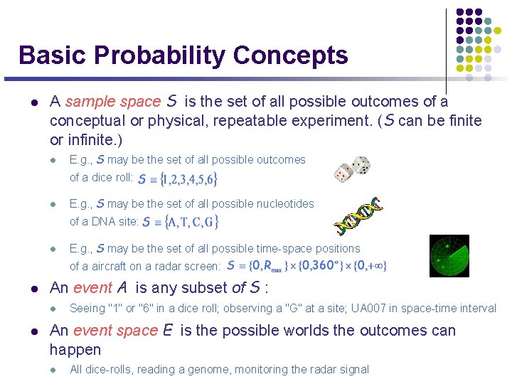
Basic Probability Concepts l A sample space S is the set of all possible outcomes of a conceptual or physical, repeatable experiment. (S can be finite or infinite. ) l E. g. , S may be the set of all possible outcomes of a dice roll: l E. g. , S may be the set of all possible nucleotides of a DNA site: l E. g. , S may be the set of all possible time-space positions of a aircraft on a radar screen: l An event A is any subset of S : l l Seeing "1" or "6" in a dice roll; observing a "G" at a site; UA 007 in space-time interval An event space E is the possible worlds the outcomes can happen l All dice-rolls, reading a genome, monitoring the radar signal

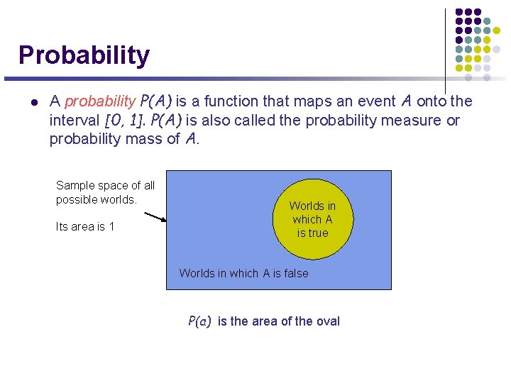
Probability l A probability P(A) is a function that maps an event A onto the interval [0, 1]. P(A) is also called the probability measure or probability mass of A. Sample space of all possible worlds. Its area is 1 Worlds in which A is true Worlds in which A is false P(a) is the area of the oval

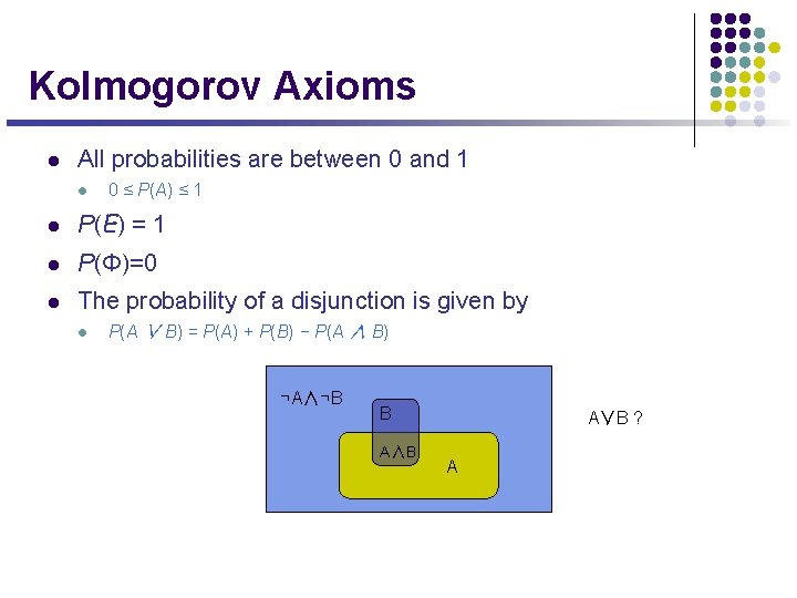
Kolmogorov Axioms l All probabilities are between 0 and 1 l 0 ≤ P(A) ≤ 1 l P(E) = 1 l P(Φ)=0 l The probability of a disjunction is given by l P(A ∨ B) = P(A) + P(B) − P(A ∧ B) ¬A∧¬B B A∧B A∨B ? A

Why use probability? l l There have been attempts to develop different methodologies for uncertainty: l Fuzzy logic l Qualitative reasoning (Qualitative physics) l … “Probability theory is nothing but common sense reduced to calculation” l l In 1931, de Finetti proved that it is irrational to have beliefs that violate these axioms, in the following sense: l l — Pierre Laplace, 1812. If you bet in accordance with your beliefs, but your beliefs violate the axioms, then you can be guaranteed to lose money to an opponent whose beliefs more accurately reflect the true state of the world. (Here, “betting” and “money” are proxies for “decision making” and “utilities”. ) What if you refuse to bet? This is like refusing to allow time to pass: every action (including inaction) is a bet

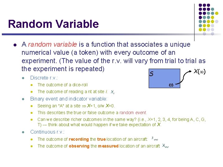
Random Variable l A random variable is a function that associates a unique numerical value (a token) with every outcome of an experiment. (The value of the r. v. will vary from trial to trial as the experiment is repeated) X(w) l l l Discrete r. v. : l The outcome of a dice-roll l The outcome of reading a nt at site i: S w Binary event and indicator variable: l Seeing an "A" at a site Þ X=1, o/w X=0. l This describes the true or false outcome a random event. l Can we describe richer outcomes in the same way? (i. e. , X=1, 2, 3, 4, for being A, C, G, T) --- think about what would happen if we take expectation of X. Continuous r. v. : l The outcome of recording the true location of an aircraft: l The outcome of observing the measured location of an aircraft

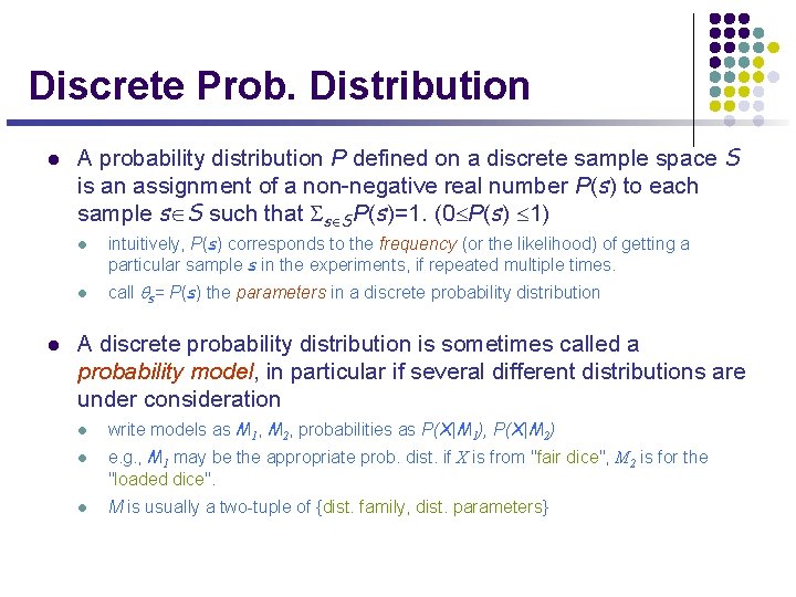
Discrete Prob. Distribution l A probability distribution P defined on a discrete sample space S is an assignment of a non-negative real number P(s) to each sample sÎS such that SsÎSP(s)=1. (0£P(s) £ 1) l l l intuitively, P(s) corresponds to the frequency (or the likelihood) of getting a particular sample s in the experiments, if repeated multiple times. call qs= P(s) the parameters in a discrete probability distribution A discrete probability distribution is sometimes called a probability model, in particular if several different distributions are under consideration l l l write models as M 1, M 2, probabilities as P(X|M 1), P(X|M 2) e. g. , M 1 may be the appropriate prob. dist. if X is from "fair dice", M 2 is for the "loaded dice". M is usually a two-tuple of {dist. family, dist. parameters}

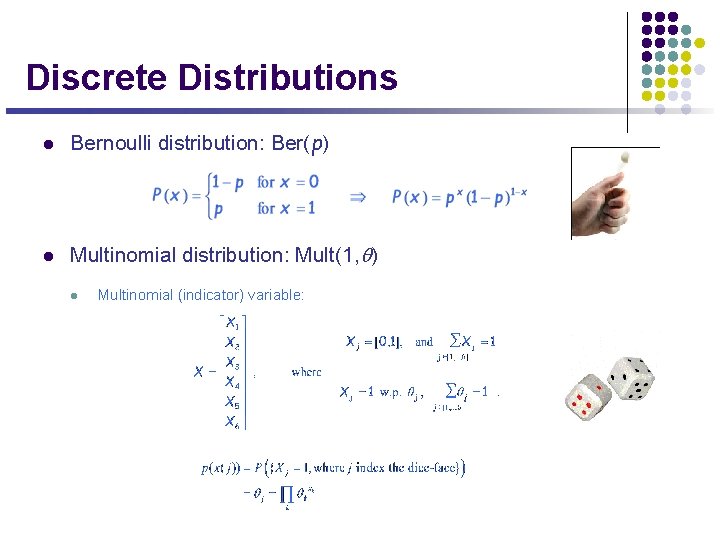
Discrete Distributions l Bernoulli distribution: Ber(p) l Multinomial distribution: Mult(1, q) l Multinomial (indicator) variable:

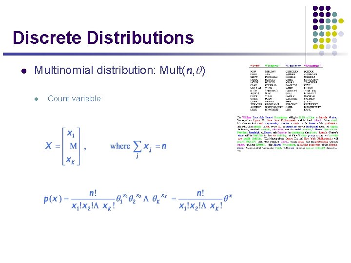
Discrete Distributions l Multinomial distribution: Mult(n, q) l Count variable:

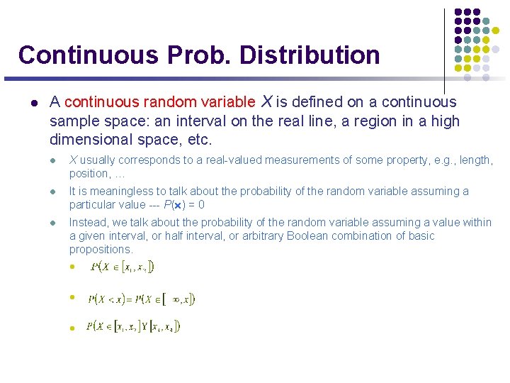
Continuous Prob. Distribution l A continuous random variable X is defined on a continuous sample space: an interval on the real line, a region in a high dimensional space, etc. l X usually corresponds to a real-valued measurements of some property, e. g. , length, position, … l It is meaningless to talk about the probability of the random variable assuming a particular value --- P(x) = 0 l Instead, we talk about the probability of the random variable assuming a value within a given interval, or half interval, or arbitrary Boolean combination of basic propositions. l l l

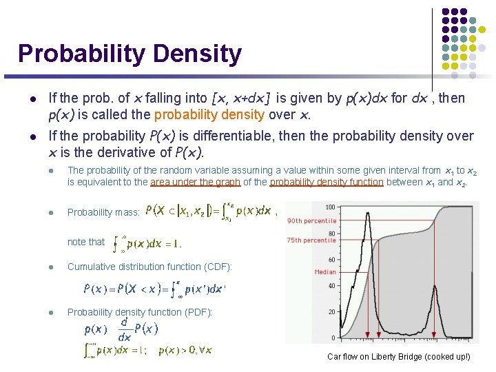
Probability Density l l If the prob. of x falling into [x, x+dx] is given by p(x)dx for dx , then p(x) is called the probability density over x. If the probability P(x) is differentiable, then the probability density over x is the derivative of P(x). l l The probability of the random variable assuming a value within some given interval from x 1 to x 2 is equivalent to the area under the graph of the probability density function between x 1 and x 2. Probability mass: note that l Cumulative distribution function (CDF): l Probability density function (PDF): Car flow on Liberty Bridge (cooked up!)

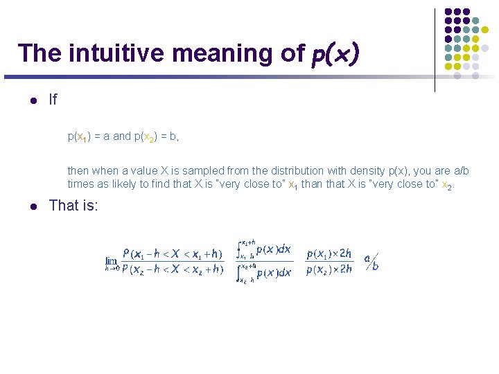
The intuitive meaning of p(x) l If p(x 1) = a and p(x 2) = b, then when a value X is sampled from the distribution with density p(x), you are a/b times as likely to find that X is “very close to” x 1 than that X is “very close to” x 2. l That is:

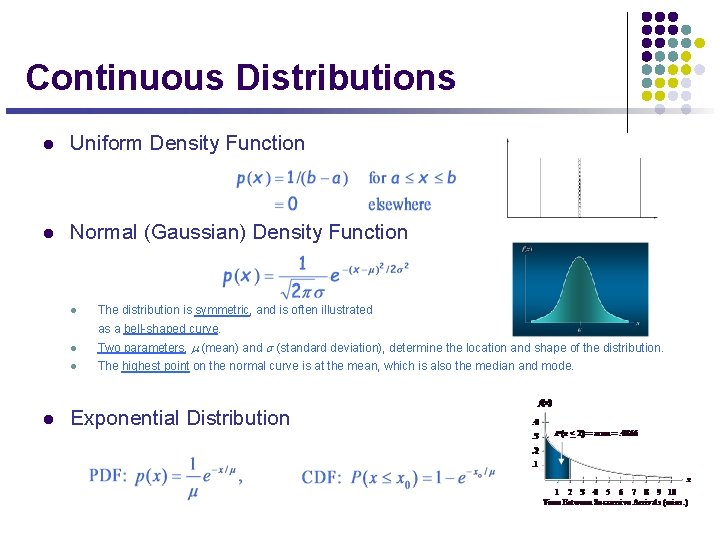
Continuous Distributions l Uniform Density Function l Normal (Gaussian) Density Function l The distribution is symmetric, and is often illustrated as a bell-shaped curve. l l Two parameters, m (mean) and s (standard deviation), determine the location and shape of the distribution. l The highest point on the normal curve is at the mean, which is also the median and mode. Exponential Distribution

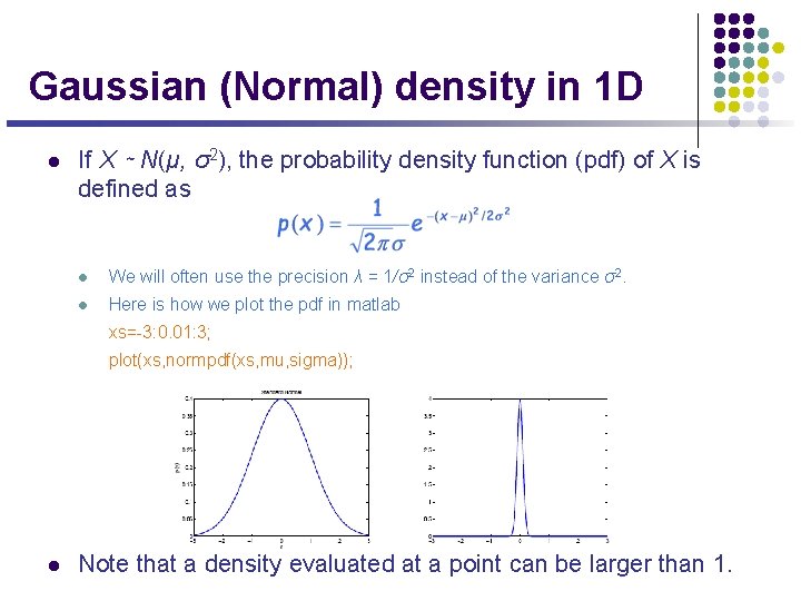
Gaussian (Normal) density in 1 D l If X ∼ N(µ, σ2), the probability density function (pdf) of X is defined as l We will often use the precision λ = 1/σ2 instead of the variance σ2. l Here is how we plot the pdf in matlab xs=-3: 0. 01: 3; plot(xs, normpdf(xs, mu, sigma)); l Note that a density evaluated at a point can be larger than 1.

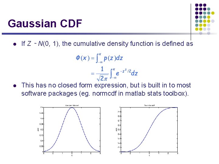
Gaussian CDF l If Z ∼ N(0, 1), the cumulative density function is defined as l This has no closed form expression, but is built in to most software packages (eg. normcdf in matlab stats toolbox).

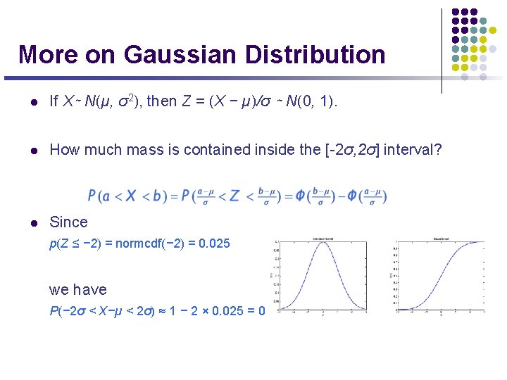
More on Gaussian Distribution l If X∼ N(µ, σ2), then Z = (X − µ)/σ ∼ N(0, 1). l How much mass is contained inside the [-2σ, 2σ] interval? l Since p(Z ≤ − 2) = normcdf(− 2) = 0. 025 we have P(− 2σ < X−µ < 2σ) ≈ 1 − 2 × 0. 025 = 0. 95

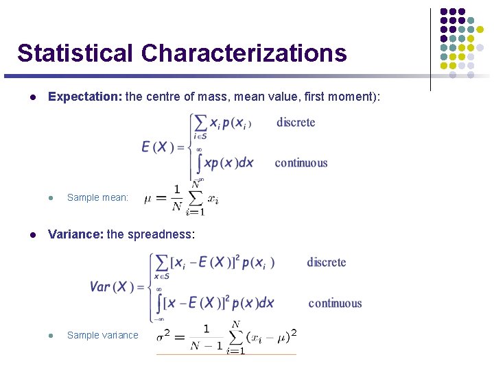
Statistical Characterizations l Expectation: the centre of mass, mean value, first moment): l l Sample mean: Variance: the spreadness: l Sample variance

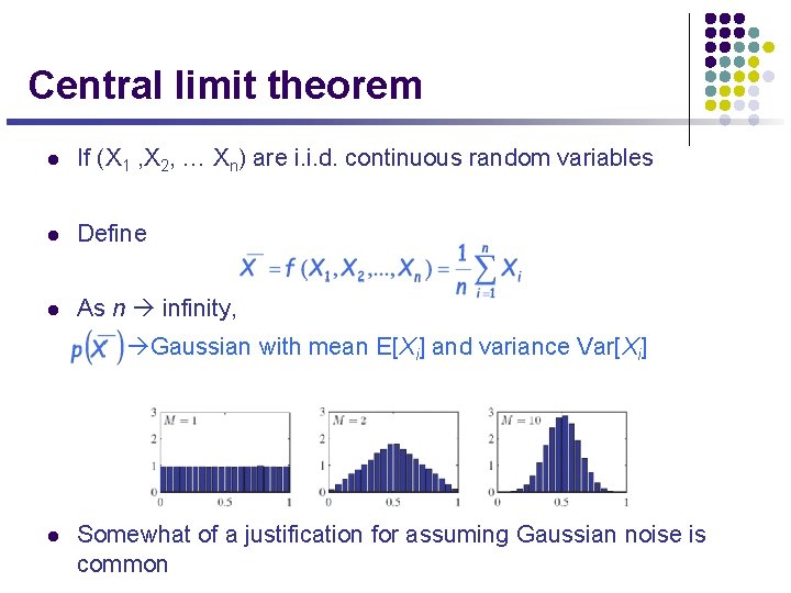
Central limit theorem l If (X 1 , X 2, … Xn) are i. i. d. continuous random variables l Define l As n infinity, Gaussian with mean E[Xi] and variance Var[Xi] l Somewhat of a justification for assuming Gaussian noise is common