M Ronen G Chandy T Meyer J E

M. Ronen, G. Chandy, T. Meyer & J. E. Ferrell

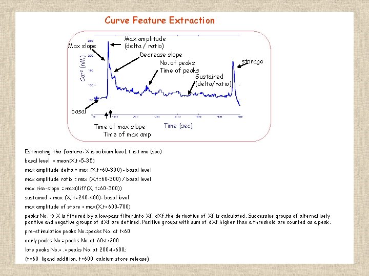
Curve Feature Extraction Ca+2 (n. M) Max slope Max amplitude (delta / ratio) Decrease slope No. of peaks Time of peaks Sustained (delta/ratio) storage basal Time of max slope Time of max amp Time (sec) Estimating the feature: X is calcium level, t is time (sec) basal level = mean(X, t=5 -35) max amplitude delta = max (X, t=60 -300) - basal level max amplitude ratio = max (X, t=60 -300) / basal level max rise-slope = max(diff(X, t=60 -300)) sustained = max (X, t=240 -480)- basal level max amplitude of store = max(X, t=600 -700) peaks No. X is filtered by a low-pass filter, into Xf. d. Xf, the derivative of Xf is calculated. Successive groups of alternatively positive and negative groups of d. Xf are defined. Positive groups with sum of d. Xf higher than a threshold are counted as a peak. pre-stimulation peaks No. =peaks No. at t<60 early peaks No. = peaks No. at 60<t<200 late peaks No. =. = peaks No. at 200<t<600; (t=60 ligand addition, t=600 calcium store release)

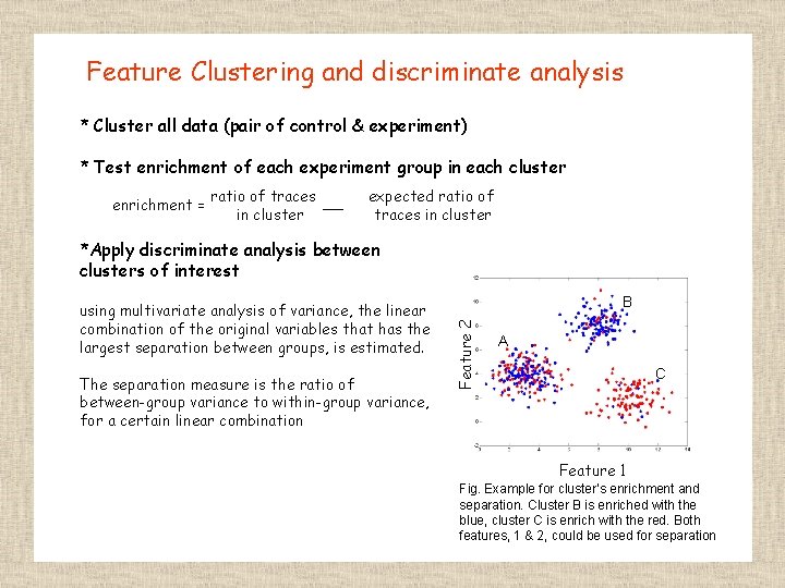
Feature Clustering and discriminate analysis * Cluster all data (pair of control & experiment) * Test enrichment of each experiment group in each cluster enrichment = ratio of traces in cluster expected ratio of traces in cluster *Apply discriminate analysis between clusters of interest The separation measure is the ratio of between-group variance to within-group variance, for a certain linear combination B Feature 2 using multivariate analysis of variance, the linear combination of the original variables that has the largest separation between groups, is estimated. A C Feature 1 Fig. Example for cluster’s enrichment and separation. Cluster B is enriched with the blue, cluster C is enrich with the red. Both features, 1 & 2, could be used for separation

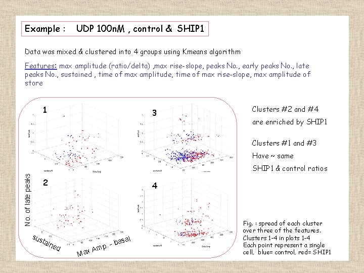
Example : UDP 100 n. M , control & SHIP 1 Data was mixed & clustered into 4 groups using Kmeans algorithm Features: max amplitude (ratio/delta) , max rise-slope, peaks No. , early peaks No. , late peaks No. , sustained , time of max amplitude, time of max rise-slope, max amplitude of store 1 3 Clusters #2 and #4 are enriched by SHIP 1 Clusters #1 and #3 Have ~ same No. of late peaks SHIP 1 & control ratios 2 4 sus tain ed Max A -b mp. asal Fig. : spread of each cluster over three of the features. Clusters 1 -4 in plots 1 -4 Each point represent a single cell, blue= control, red= SHIP 1

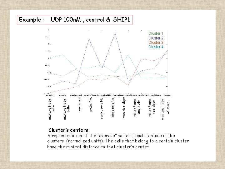
UDP 100 n. M , control & SHIP 1 Cluster’s centers of store max amplitude time of max rise-slope time of max amplitude max rise-slope late peaks No. early peaks No. sustained max amplitude delta Cluster 1 Cluster 2 Cluster 3 Cluster 4 max amplitude ratio Example : A representation of the “average” value of each feature in the clusters (normalized units). The cells that belong to a certain cluster have the minimal distance to that cluster’s center.

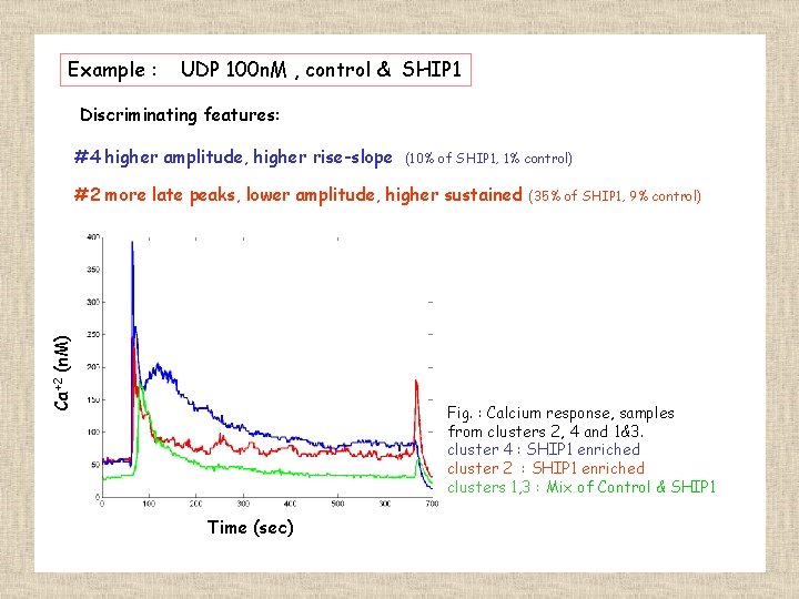
Example : UDP 100 n. M , control & SHIP 1 Discriminating features: #4 higher amplitude, higher rise-slope (10% of SHIP 1, 1% control) Ca+2 (n. M) #2 more late peaks, lower amplitude, higher sustained (35% of SHIP 1, 9% control) Fig. : Calcium response, samples from clusters 2, 4 and 1&3. cluster 4 : SHIP 1 enriched cluster 2 : SHIP 1 enriched clusters 1, 3 : Mix of Control & SHIP 1 Time (sec)

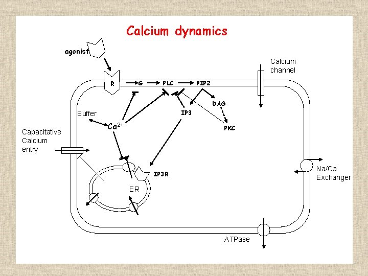
Calcium dynamics agonist Calcium channel R G PLC PIP 2 DAG IP 3 Buffer Capacitative Calcium entry Ca 2+ PKC Na/Ca Exchanger IP 3 R ER ATPase

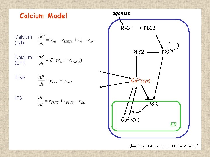
Calcium Model agonist R-G PLCβ Calcium (cyt) Calcium (ER) IP 3 R IP 3 PLCδ Ca 2+(cyt) IP 3 R Ca 2+(ER) ER (based on Hofer et al. , J. Neuro. , 22, 4850)

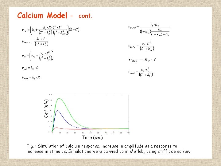
Ca+2 (u. M) Calcium Model - cont. Time (sec) Fig. : Simulation of calcium response, increase in amplitude as a response to increase in stimulus. Simulations were carried up in Matlab, using stiff ode solver.

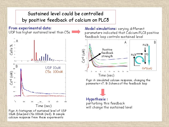
Sustained level could be controlled by positive feedback of calcium on PLCδ From experimental data: UDP has higher sustained level than C 5 a A parameters indicated that Calcium-PLCd positive feedback loop controls sustained level A Ca+2 (u. M) Cells % B Ca+2 (n. M) Model simulations: varying different UDP 10 u. M C 5 a 100 n. M Positive feedback strength PLCβ PLCδ IP 3 Ca 2+(cyt) Time (sec) Figs: A: simulated calcium response, changing the parameter v 7. B: Schema of the feedback loop Hypothesis : Time (sec) Figs: A: histogram of sustained level of UDP 10 u. M (blue)and C 5 a 100 n. M (red). B: sample calcium response from these experiments perturbing this feedback will change the sustained level B

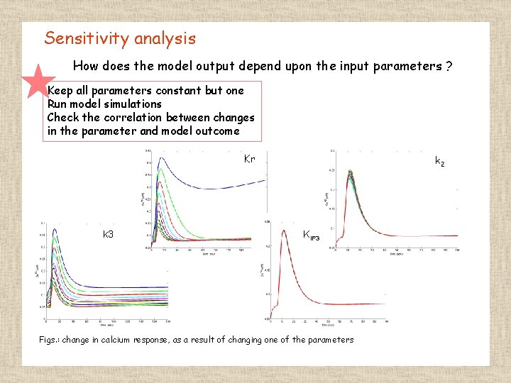
Sensitivity analysis How does the model output depend upon the input parameters ? Keep all parameters constant but one Run model simulations Check the correlation between changes in the parameter and model outcome Kr k 3 K 3 k 2 KIP 3 k. IP 3 Figs. : change in calcium response, as a result of changing one of the parameters

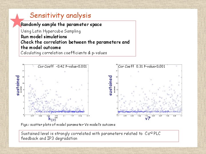
Sensitivity analysis Randomly sample the parameter space Using Latin Hypercube Sampling Run model simulations Check the correlation between the parameters and the model outcome Calculating correlation coefficients & p-values Cor Coeff 0. 31 P-value<0. 001 sustained Cor Coeff -0. 42 P-value<0. 001 k. IP 3 v 7 Figs. : scatter plots of model parameter Vs model’s outcome Sustained level is strongly correlated with parameters related to Ca +2 PLC feedback and IP 3 degradation

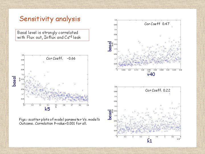
Sensitivity analysis Cor Coeff 0. 47 basal Basal level is strongly correlated with Flux out, Influx and Ca+2 leak Cor Coeff. -0. 66 basal v 40 k 5 Figs. : scatter plots of model parameter Vs. model’s Outcome. Correlation P-value<0. 001 for all. basal Cor Coeff. 0. 22 k 1

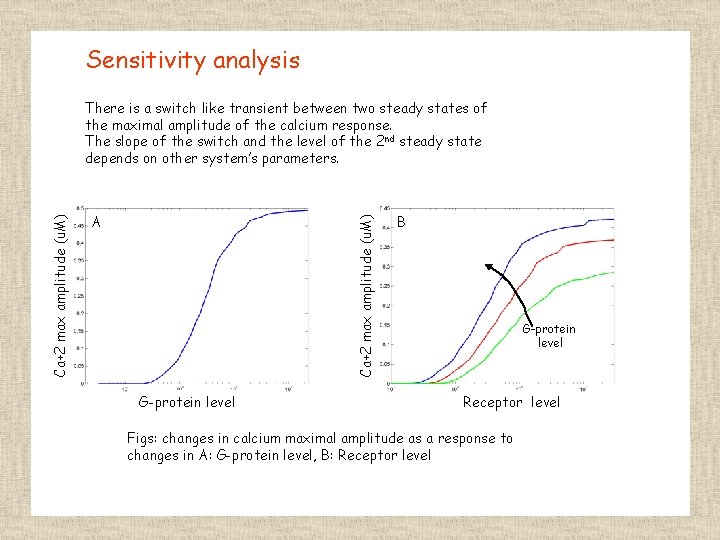
Sensitivity analysis A Ca+2 max amplitude (u. M) There is a switch like transient between two steady states of the maximal amplitude of the calcium response. The slope of the switch and the level of the 2 nd steady state depends on other system’s parameters. G-protein level B G-protein level Receptor level Figs: changes in calcium maximal amplitude as a response to changes in A: G-protein level, B: Receptor level