Linear Regression Industrial Engineering Majors Authors Autar Kaw

Linear Regression Industrial Engineering Majors Authors: Autar Kaw, Luke Snyder http: //numericalmethods. eng. usf. edu Transforming Numerical Methods Education for STEM Undergraduates 11/10/2020 http: //numericalmethods. eng. usf. edu 1

Linear Regression http: //numericalmethods. eng. usf. edu

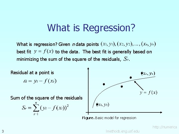
What is Regression? What is regression? Given n data points best fit to the data. The best fit is generally based on minimizing the sum of the square of the residuals, . Residual at a point is Sum of the square of the residuals Figure. Basic model for regression 3 http: //numerica lmethods. eng. usf. edu

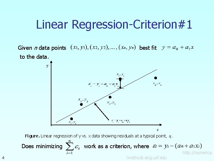
Linear Regression-Criterion#1 Given n data points best fit to the data. y x Figure. Linear regression of y vs. x data showing residuals at a typical point, xi. Does minimizing 4 work as a criterion, where http: //numerica lmethods. eng. usf. edu

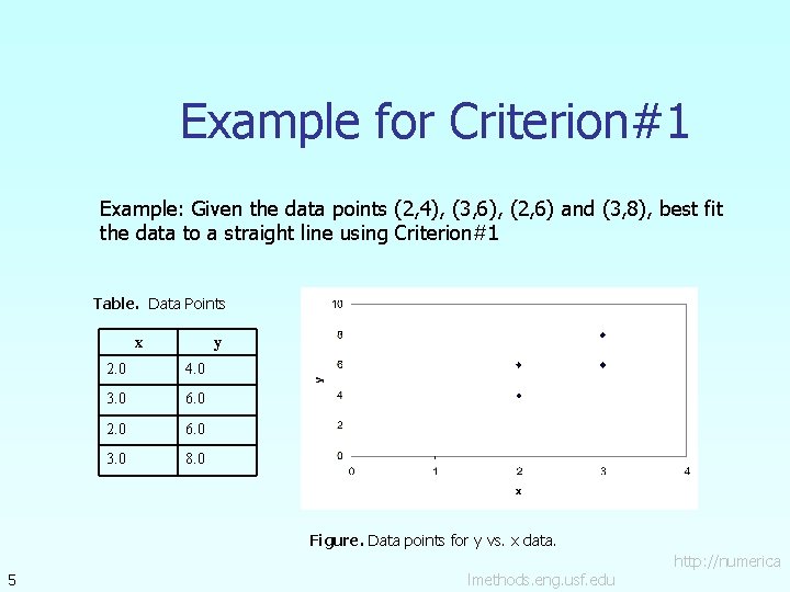
Example for Criterion#1 Example: Given the data points (2, 4), (3, 6), (2, 6) and (3, 8), best fit the data to a straight line using Criterion#1 Table. Data Points x 5 y 2. 0 4. 0 3. 0 6. 0 2. 0 6. 0 3. 0 8. 0 Figure. Data points for y vs. x data. http: //numerica lmethods. eng. usf. edu

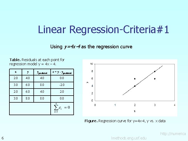
Linear Regression-Criteria#1 Using y=4 x-4 as the regression curve Table. Residuals at each point for regression model y = 4 x – 4. x y ypredicted ε = y - ypredicted 2. 0 4. 0 0. 0 3. 0 6. 0 8. 0 -2. 0 6. 0 4. 0 2. 0 3. 0 8. 0 0. 0 Figure. Regression curve for y=4 x-4, y vs. x data 6 http: //numerica lmethods. eng. usf. edu

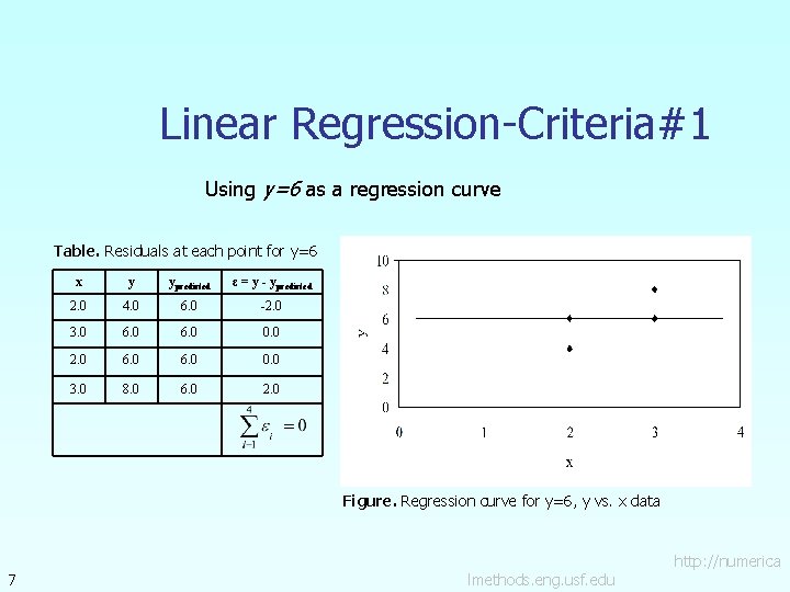
Linear Regression-Criteria#1 Using y=6 as a regression curve Table. Residuals at each point for y=6 x y ypredicted ε = y - ypredicted 2. 0 4. 0 6. 0 -2. 0 3. 0 6. 0 0. 0 2. 0 6. 0 0. 0 3. 0 8. 0 6. 0 2. 0 Figure. Regression curve for y=6, y vs. x data 7 http: //numerica lmethods. eng. usf. edu

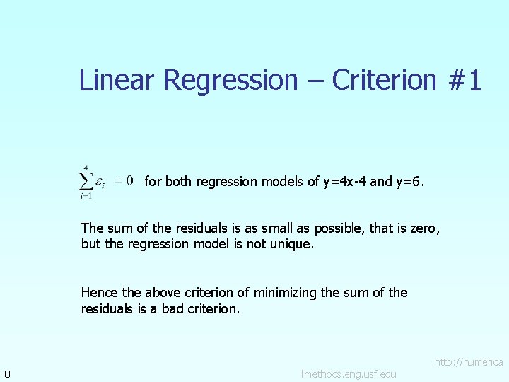
Linear Regression – Criterion #1 for both regression models of y=4 x-4 and y=6. The sum of the residuals is as small as possible, that is zero, but the regression model is not unique. Hence the above criterion of minimizing the sum of the residuals is a bad criterion. 8 http: //numerica lmethods. eng. usf. edu

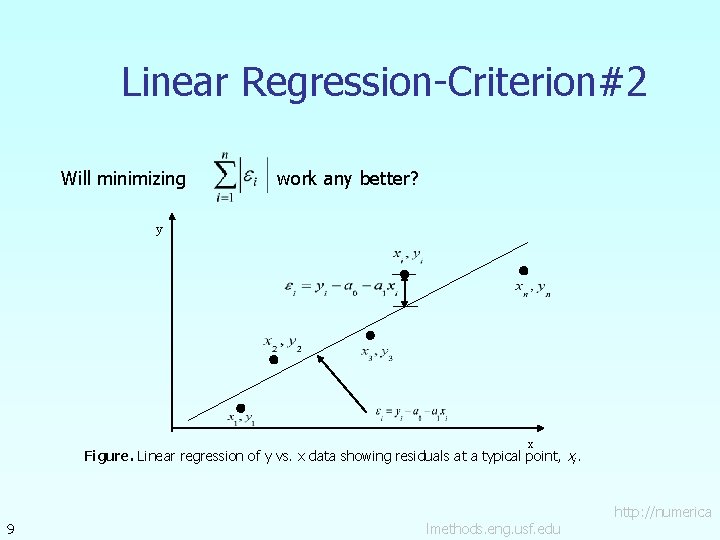
Linear Regression-Criterion#2 Will minimizing work any better? y x Figure. Linear regression of y vs. x data showing residuals at a typical point, xi. 9 http: //numerica lmethods. eng. usf. edu

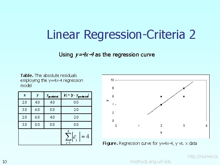
Linear Regression-Criteria 2 Using y=4 x-4 as the regression curve Table. The absolute residuals employing the y=4 x-4 regression model x y ypredicted |ε| = |y - ypredicted| 2. 0 4. 0 0. 0 3. 0 6. 0 8. 0 2. 0 6. 0 4. 0 2. 0 3. 0 8. 0 0. 0 Figure. Regression curve for y=4 x-4, y vs. x data 10 http: //numerica lmethods. eng. usf. edu

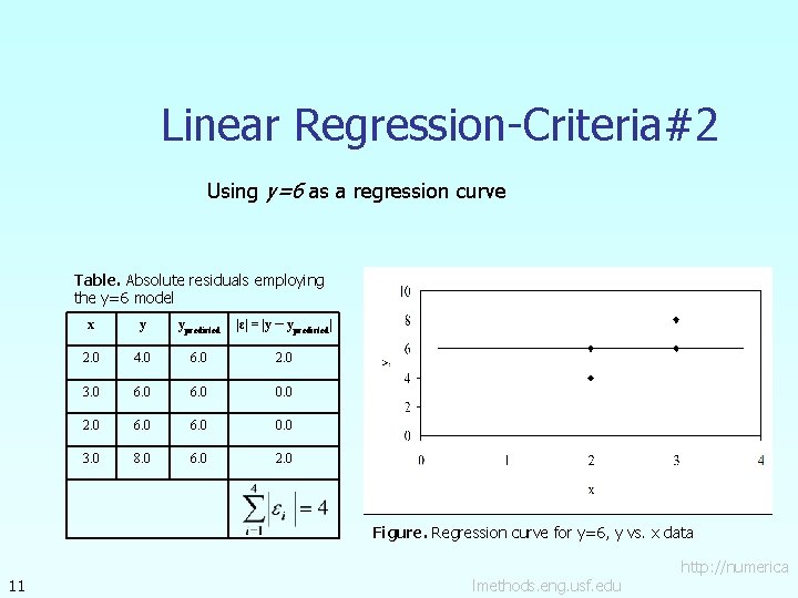
Linear Regression-Criteria#2 Using y=6 as a regression curve Table. Absolute residuals employing the y=6 model x y ypredicted |ε| = |y – ypredicted| 2. 0 4. 0 6. 0 2. 0 3. 0 6. 0 0. 0 2. 0 6. 0 0. 0 3. 0 8. 0 6. 0 2. 0 Figure. Regression curve for y=6, y vs. x data 11 http: //numerica lmethods. eng. usf. edu

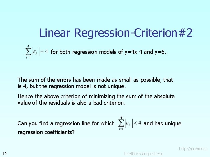
Linear Regression-Criterion#2 for both regression models of y=4 x-4 and y=6. The sum of the errors has been made as small as possible, that is 4, but the regression model is not unique. Hence the above criterion of minimizing the sum of the absolute value of the residuals is also a bad criterion. Can you find a regression line for which and has unique regression coefficients? 12 http: //numerica lmethods. eng. usf. edu

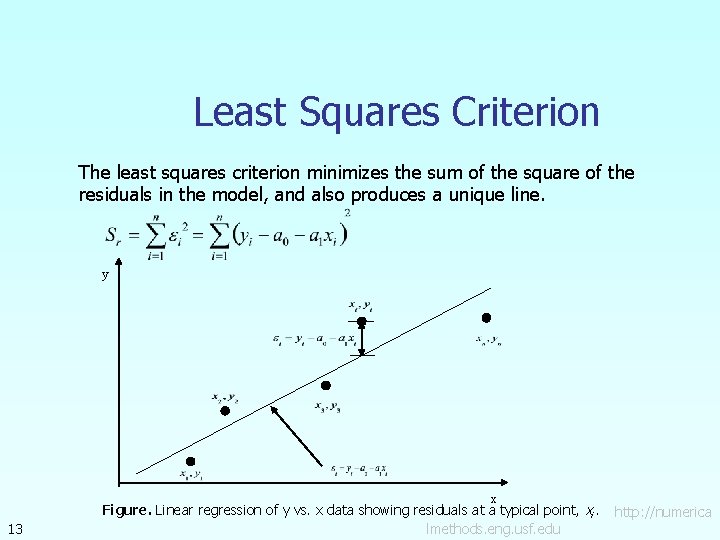
Least Squares Criterion The least squares criterion minimizes the sum of the square of the residuals in the model, and also produces a unique line. y x 13 Figure. Linear regression of y vs. x data showing residuals at a typical point, xi. http: //numerica lmethods. eng. usf. edu

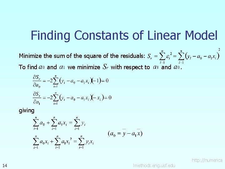
Finding Constants of Linear Model Minimize the sum of the square of the residuals: To find and we minimize with respect to and . giving 14 http: //numerica lmethods. eng. usf. edu

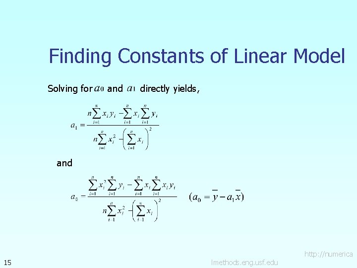
Finding Constants of Linear Model Solving for and directly yields, and 15 http: //numerica lmethods. eng. usf. edu

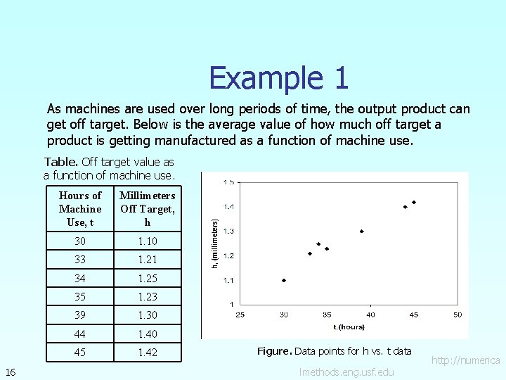
Example 1 As machines are used over long periods of time, the output product can get off target. Below is the average value of how much off target a product is getting manufactured as a function of machine use. Table. Off target value as a function of machine use. 16 Hours of Machine Use, t Millimeters Off Target, h 30 1. 10 33 1. 21 34 1. 25 35 1. 23 39 1. 30 44 1. 40 45 1. 42 Figure. Data points for h vs. t data http: //numerica lmethods. eng. usf. edu

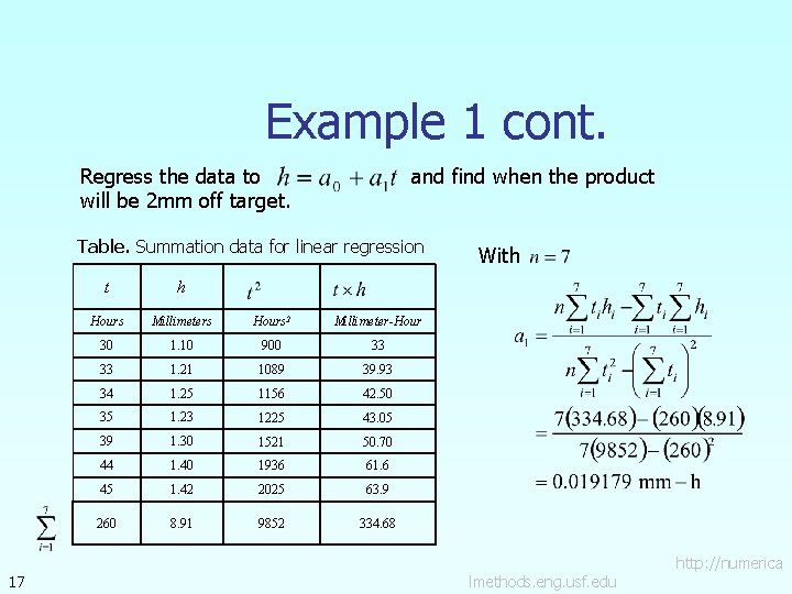
Example 1 cont. Regress the data to and find when the product will be 2 mm off target. Table. Summation data for linear regression 17 t h Hours Millimeters Hours 2 Millimeter-Hour 30 1. 10 900 33 33 1. 21 1089 39. 93 34 1. 25 1156 42. 50 35 1. 23 1225 43. 05 39 1. 30 1521 50. 70 44 1. 40 1936 61. 6 45 1. 42 2025 63. 9 260 8. 91 9852 334. 68 With http: //numerica lmethods. eng. usf. edu

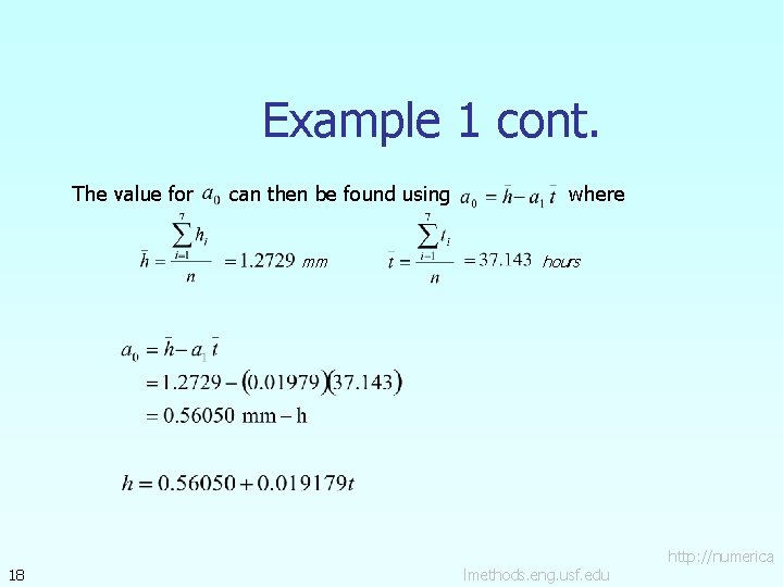
Example 1 cont. The value for can then be found using mm 18 where hours http: //numerica lmethods. eng. usf. edu

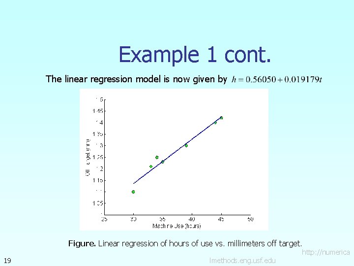
Example 1 cont. The linear regression model is now given by Figure. Linear regression of hours of use vs. millimeters off target. 19 http: //numerica lmethods. eng. usf. edu

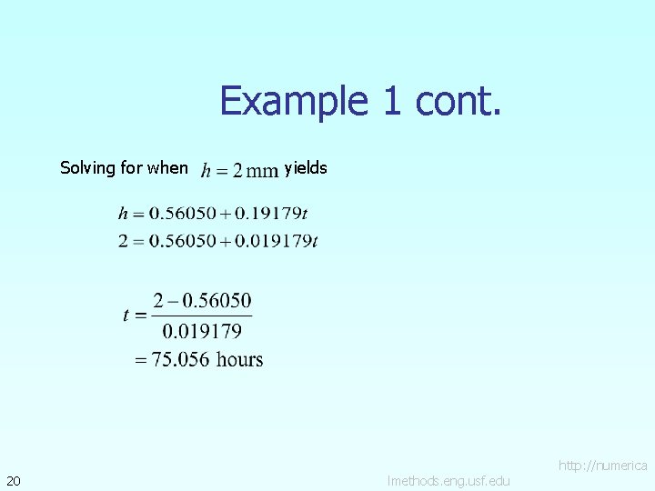
Example 1 cont. Solving for when 20 yields http: //numerica lmethods. eng. usf. edu

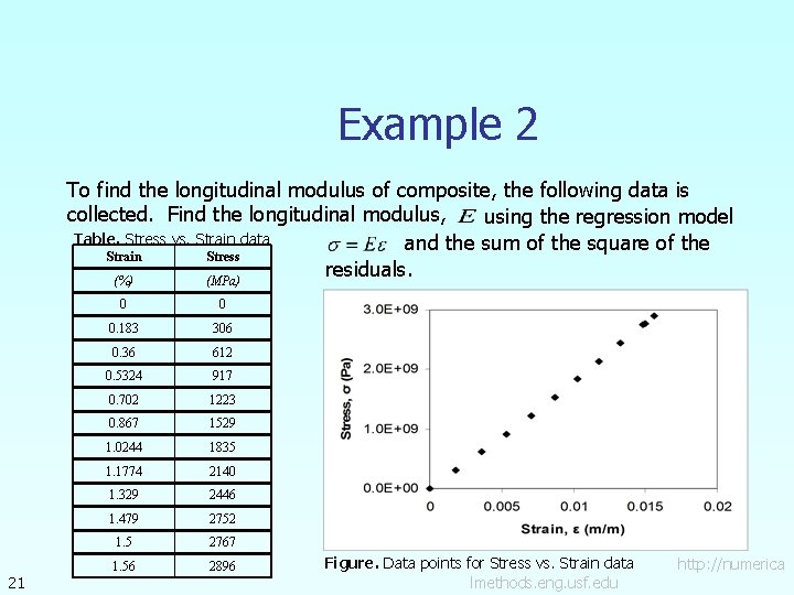
Example 2 To find the longitudinal modulus of composite, the following data is collected. Find the longitudinal modulus, using the regression model Table. Stress vs. Strain data and the sum of the square of the Strain Stress residuals. (%) (MPa) 21 0 0 0. 183 306 0. 36 612 0. 5324 917 0. 702 1223 0. 867 1529 1. 0244 1835 1. 1774 2140 1. 329 2446 1. 479 2752 1. 5 2767 1. 56 2896 Figure. Data points for Stress vs. Strain data http: //numerica lmethods. eng. usf. edu

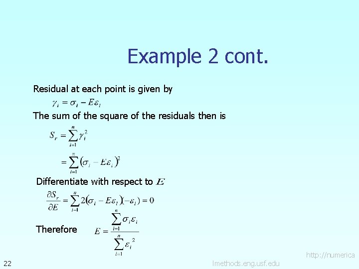
Example 2 cont. Residual at each point is given by The sum of the square of the residuals then is Differentiate with respect to Therefore 22 http: //numerica lmethods. eng. usf. edu

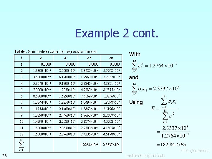
Example 2 cont. Table. Summation data for regression model 23 i ε σ ε 2 εσ 1 0. 0000 2 1. 8300× 10− 3 3. 0600× 108 3. 3489× 10− 6 5. 5998× 105 3 3. 6000× 10− 3 6. 1200× 108 1. 2960× 10− 5 2. 2032× 106 4 5. 3240× 10− 3 9. 1700× 108 2. 8345× 10− 5 4. 8821× 106 5 7. 0200× 10− 3 1. 2230× 109 4. 9280× 10− 5 8. 5855× 106 6 8. 6700× 10− 3 1. 5290× 109 7. 5169× 10− 5 1. 3256× 107 7 1. 0244× 10− 2 1. 8350× 109 1. 0494× 10− 4 1. 8798× 107 8 1. 1774× 10− 2 2. 1400× 109 1. 3863× 10− 4 2. 5196× 107 9 1. 3290× 10− 2 2. 4460× 109 1. 7662× 10− 4 3. 2507× 107 10 1. 4790× 10− 2 2. 7520× 109 2. 1874× 10− 4 4. 0702× 107 11 1. 5000× 10− 2 2. 7670× 109 2. 2500× 10− 4 4. 1505× 107 12 1. 5600× 10− 2 2. 8960× 109 2. 4336× 10− 4 4. 5178× 107 1. 2764× 10− 3 2. 3337× 108 With and Using http: //numerica lmethods. eng. usf. edu

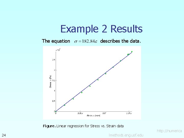
Example 2 Results The equation 24 describes the data. Figure. Linear regression for Stress vs. Strain data http: //numerica lmethods. eng. usf. edu

Additional Resources For all resources on this topic such as digital audiovisual lectures, primers, textbook chapters, multiple-choice tests, worksheets in MATLAB, MATHEMATICA, Math. Cad and MAPLE, blogs, related physical problems, please visit http: //numericalmethods. eng. usf. edu/topics/linear_regr ession. html

THE END http: //numericalmethods. eng. usf. edu