Last Update 17 th June 2011 SESSION 49

Last Update 17 th June 2011 SESSION 49 - 52 Regression

Lecturer: University: Domain: Florian Boehlandt University of Stellenbosch Business School http: //www. hedge-fundanalysis. net/pages/vega. php

Learning Objectives 1. 2. 3. 4. 5. XY-Scatter Diagrams Plotting the Regression Line Coefficient Estimates Pearson Coefficient of Correlation Spearman Rank Correlation Coefficient

XY-Scatter Diagram To draw a scatter diagram we need data for two variables. In applications where one variable depends to some degree on the other variable, the dependent variable is labeled Y and the other, called the independent variable, X. The values for X and Y are combined into a single data point using the observations for X and Y as coordinates.

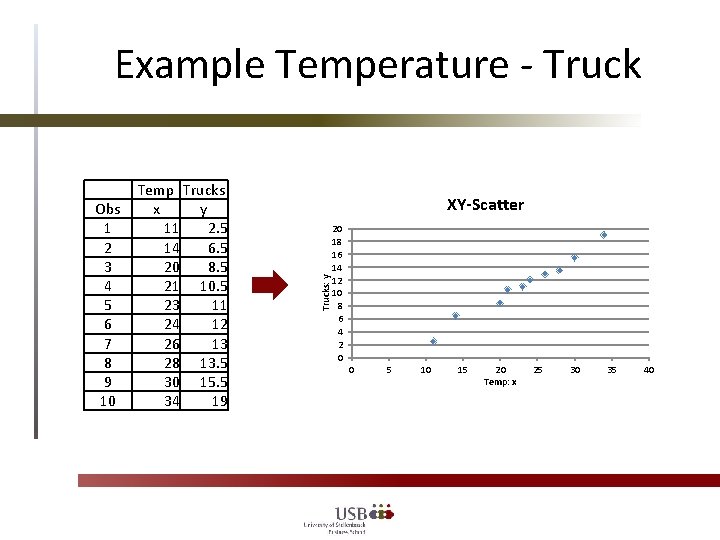
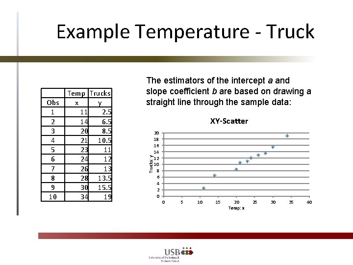
Example Temperature - Truck XY-Scatter Trucks: y Obs 1 2 3 4 5 6 7 8 9 10 Temp Trucks x y 11 2. 5 14 6. 5 20 8. 5 21 10. 5 23 11 24 12 26 13 28 13. 5 30 15. 5 34 19 20 18 16 14 12 10 8 6 4 2 0 0 5 10 15 20 Temp: x 25 30 35 40

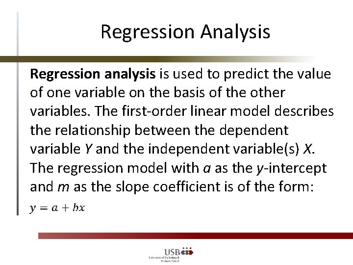
Regression Analysis Regression analysis is used to predict the value of one variable on the basis of the other variables. The first-order linear model describes the relationship between the dependent variable Y and the independent variable(s) X. The regression model with a as the y-intercept and m as the slope coefficient is of the form:

Example Temperature - Truck XY-Scatter Trucks: y Obs 1 2 3 4 5 6 7 8 9 10 Temp Trucks x y 11 2. 5 14 6. 5 20 8. 5 21 10. 5 23 11 24 12 26 13 28 13. 5 30 15. 5 34 19 The estimators of the intercept a and slope coefficient b are based on drawing a straight line through the sample data: 20 18 16 14 12 10 8 6 4 2 0 0 5 10 15 20 Temp: x 25 30 35 40

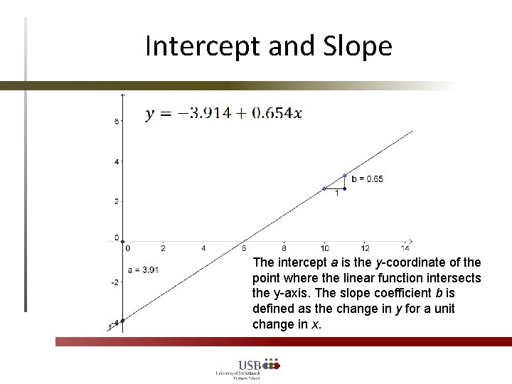
Intercept and Slope The intercept a is the y-coordinate of the point where the linear function intersects the y-axis. The slope coefficient b is defined as the change in y for a unit change in x.

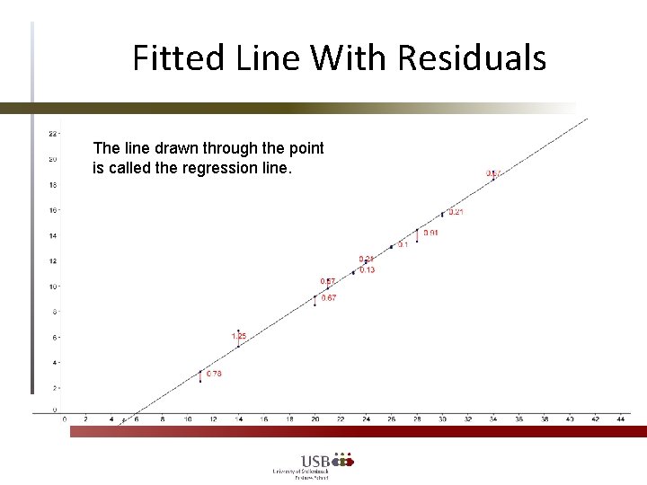
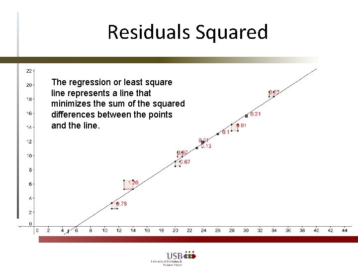
Fitted Line With Residuals The line drawn through the point is called the regression line.

Residuals Squared The regression or least square line represents a line that minimizes the sum of the squared differences between the points and the line.

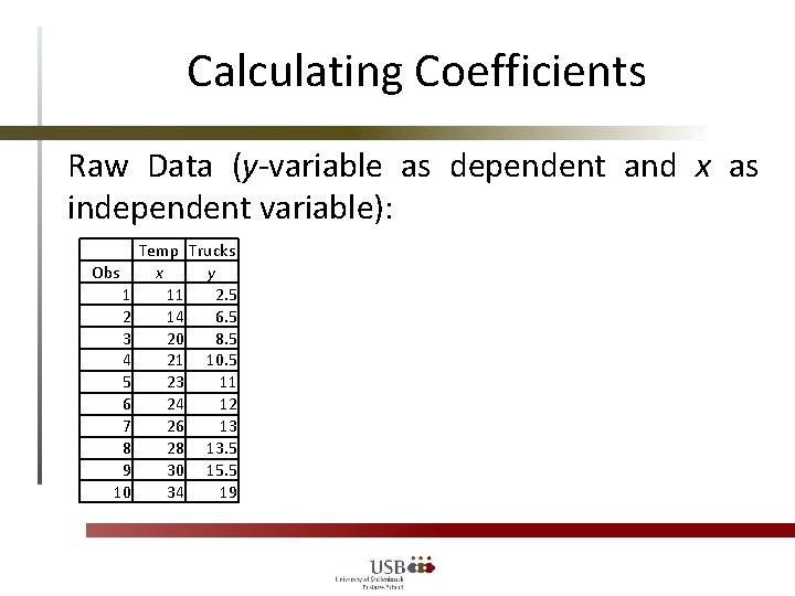
Calculating Coefficients Raw Data (y-variable as dependent and x as independent variable): Obs 1 2 3 4 5 6 7 8 9 10 Temp Trucks x y 11 2. 5 14 6. 5 20 8. 5 21 10. 5 23 11 24 12 26 13 28 13. 5 30 15. 5 34 19

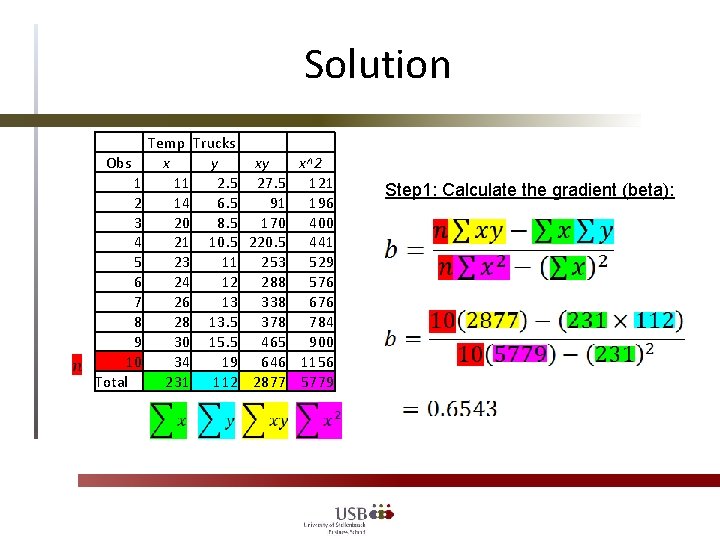
Solution Obs 1 2 3 4 5 6 7 8 9 10 Total Temp Trucks x y xy x^2 11 2. 5 27. 5 121 14 6. 5 91 196 20 8. 5 170 400 21 10. 5 220. 5 441 23 11 253 529 24 12 288 576 26 13 338 676 28 13. 5 378 784 30 15. 5 465 900 34 19 646 1156 231 112 2877 5779 Step 1: Calculate the gradient (beta):

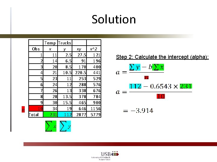
Solution Obs 1 2 3 4 5 6 7 8 9 10 Total Temp Trucks x y xy x^2 11 2. 5 27. 5 121 14 6. 5 91 196 20 8. 5 170 400 21 10. 5 220. 5 441 23 11 253 529 24 12 288 576 26 13 338 676 28 13. 5 378 784 30 15. 5 465 900 34 19 646 1156 231 112 2877 5779 Step 2: Calculate the intercept (alpha):

Interpreting the Coefficients The slope coefficient b may be interpreted as the change in the dependent variable y for a one unit change in x. In the previous example, a one unit change in temperature results in a b = 0. 654 additional truckloads of cool drinks sold. The intercept a is the point at which the regression line and the y -axis intersect. If x = 0 lies far outside the range of sample values x, the interpretation of the intercept is not straight-forward. In the temperature-truck example, x = 0 lies outside the smallest and largest values for x in the sample. Interpreting the intercept for x would imply that at temperature of x = 0, the soft-drink sales decline to negative 3. 914!

Point Prediction Upon obtaining the coefficient estimates we can predict the outcome for various x (point prediction) between the minimum and maximum sample observation using the regression function y = a + mx. For example: x = 16 degrees? y = 3. 914 + 0. 654*16 y = 6. 554 ≈ 7 truckloads X = 32 degrees? y = 3. 914 + 0. 654*32 y = 17. 023 ≈ 17 truckloads

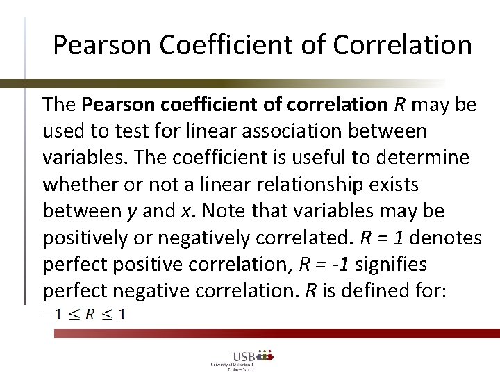
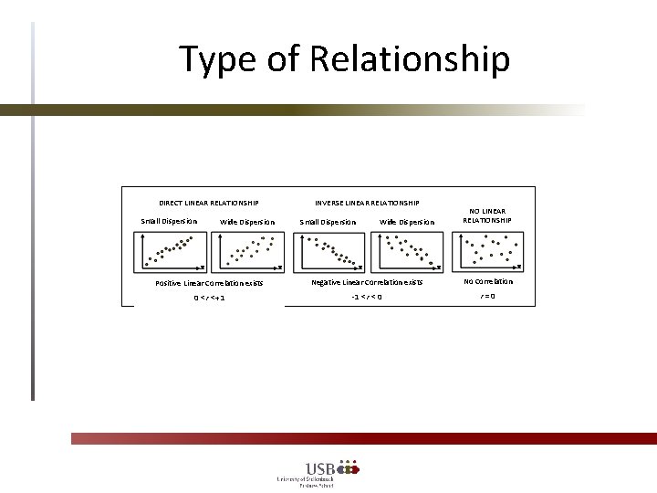
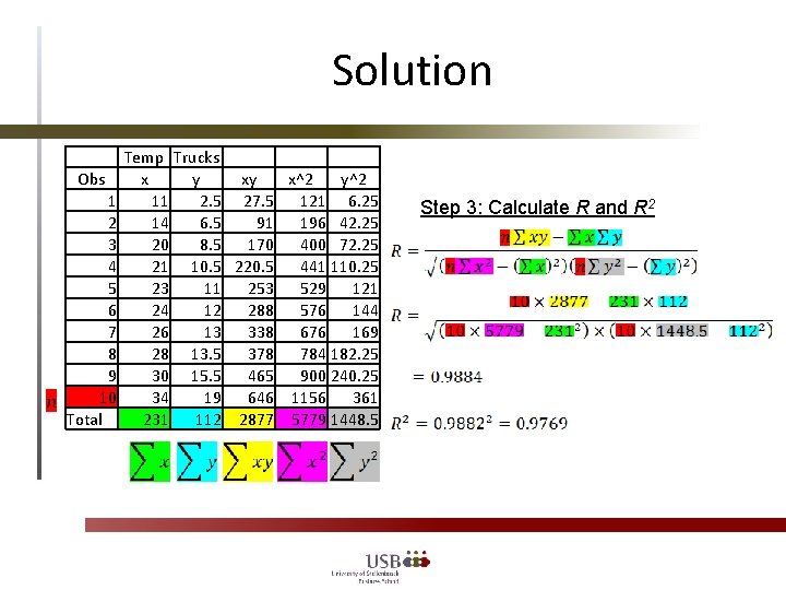
Pearson Coefficient of Correlation The Pearson coefficient of correlation R may be used to test for linear association between variables. The coefficient is useful to determine whether or not a linear relationship exists between y and x. Note that variables may be positively or negatively correlated. R = 1 denotes perfect positive correlation, R = -1 signifies perfect negative correlation. R is defined for:

Type of Relationship DIRECT LINEAR RELATIONSHIP Small Dispersion Wide Dispersion INVERSE LINEAR RELATIONSHIP Small Dispersion Wide Dispersion NO LINEAR RELATIONSHIP Positive Linear Correlation exists Negative Linear Correlation exists No Correlation 0 < r <+ 1 -1 < r < 0 r=0

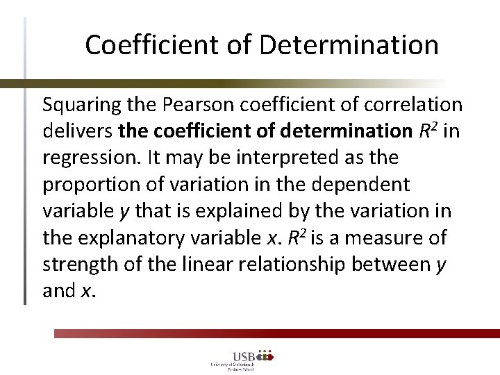
Coefficient of Determination Squaring the Pearson coefficient of correlation delivers the coefficient of determination R 2 in regression. It may be interpreted as the proportion of variation in the dependent variable y that is explained by the variation in the explanatory variable x. R 2 is a measure of strength of the linear relationship between y and x.

Solution Obs 1 2 3 4 5 6 7 8 9 10 Total Temp Trucks x y xy x^2 y^2 11 2. 5 27. 5 121 6. 25 14 6. 5 91 196 42. 25 20 8. 5 170 400 72. 25 21 10. 5 220. 5 441 110. 25 23 11 253 529 121 24 12 288 576 144 26 13 338 676 169 28 13. 5 378 784 182. 25 30 15. 5 465 900 240. 25 34 19 646 1156 361 231 112 2877 5779 1448. 5 Step 3: Calculate R and R 2

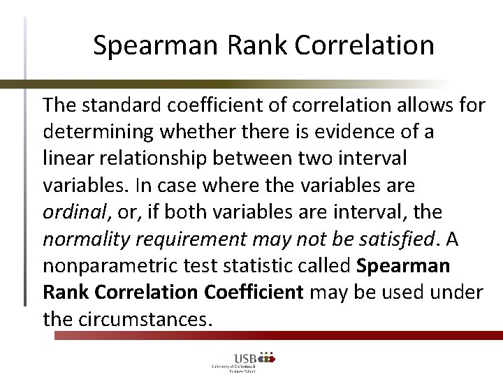
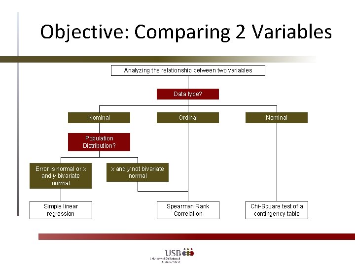
Spearman Rank Correlation The standard coefficient of correlation allows for determining whethere is evidence of a linear relationship between two interval variables. In case where the variables are ordinal, or, if both variables are interval, the normality requirement may not be satisfied. A nonparametric test statistic called Spearman Rank Correlation Coefficient may be used under the circumstances.

Objective: Comparing 2 Variables Analyzing the relationship between two variables Data type? Nominal Ordinal Nominal Spearman Rank Correlation Chi-Square test of a contingency table Population Distribution? Error is normal or x and y bivariate normal Simple linear regression x and y not bivariate normal

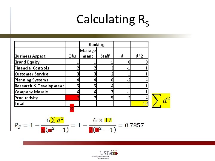
Example Below there is a list of organizational strengths that were independently ranked by management and staff and the managing director wished to know how closely correlated were the assessments: Ranking Manag Business Aspect ement Staff Brand Equity 1 1 Financial Controls 2 3 Customer Service 3 2 Planning Systems 4 6 Research & Development 5 4 Company Morale 6 7 Productivity 7 5

Calculating RS Ranking Manage Business Aspect Obs ment Staff Brand Equity 1 1 Financial Controls 2 2 Customer Service 3 3 Planning Systems 4 4 Research & Development 5 5 Company Morale 6 6 Productivity 7 7 Total d 1 3 2 6 4 7 5 d^2 0 -1 1 -2 1 -1 2 0 1 1 4 12